Abstracts
Abstract
In this work we present a case study of the multi-scale calibration and validation of MHYDAS-Erosion applied to a Mediterranean vineyard. The calibration was performed using expert knowledge in linking physical parameters to land uses with the automatic parameter estimation software PEST. MHYDAS-Erosion was calibrated and validated using spatially distributed observations on total discharge and soil loss. Calibration has been performed within six rainfall events; both hydrological and erosion parameters were calibrated using RMSE, R2 and the modified version of the Nash-Sutcliffe model efficiency criteria. Calibration results indicate there was good agreement between simulated and observed total discharge and total soil loss at the seven observation points (modified Nash-Sutcliffe efficiency (mNSE) ranging between 0.89 and 0.95). Acceptable results were obtained in terms of parameter values, identification of their physical meaning and coherence. However, some limitations were also identified, and could be remedied in more detailed studies involving (i) spatially-distributed rainfall on the catchment, (ii) a description of groundwater exfiltration and (iii) spatially-distributed properties of the ditches over the catchment. Validation results were quite satisfactory for three of the four validation events. The results from this case study suggest that MHYDAS-Erosion may need a specific calibration when applied to another catchment, but once it is calibrated, it could be used for multi-scale soil loss forecasting.
Keywords:
- erosion modelling,
- soil loss,
- hydrological processes,
- calibration and validation,
- PEST,
- MHYDAS-Erosion
Résumé
Ce travail présente une étude de cas qui traite du calage et de la validation multiéchelle du modèle MHYDAS-Erosion appliqué au bassin versant de Roujan, en France, occupé principalement par des vignobles. Pour le calage, les valeurs des paramètres touchant les cultures ont été estimées à partir des connaissances d’experts et du logiciel d’estimation des paramètres PEST. Des mesures de débits en rivière et de pertes de sol ont ensuite servi à caler le modèle. Six événements ont servi à effectuer le calage du modèle, et quatre ont été utilisés pour valider ce calage. L’intégrité physique des valeurs des paramètres a été respectée. Les résultats du calage indiquent que le modèle est très fidèle aux données observées pour sept points de contrôle distribués sur le bassin versant de Roujan. Les résultats de validation de MHYDAS-Erosion sur le bassin versant de Roujan sont acceptables pour trois des quatre événements choisis. Quelques éléments dans la procédure de calage du modèle pourraient être améliorés au cours d’études subséquentes. Notamment, nous avons constaté que les précipitations varient beaucoup dans le bassin versant de Roujan, et qu’il serait important de considérer cette variation spatiale pour des applications futures du modèle. Aussi, comme les écoulements hypodermiques représentent une grande partie du débit à l’exutoire du bassin versant pour certains événements, il serait préférable de spatialiser les propriétés du réseau de fossés de drainage plutôt que de les considérer uniformes sur l’ensemble du bassin, comme dans la présente étude. L’utilisation du modèle MHYDAS-Erosion sur un autre bassin versant nécessiterait un calage préalable de la valeur des paramètres. Une fois calé, le modèle permettrait d’estimer les pertes de sol pour différents secteurs du bassin versant. Il pourrait aussi servir à tester des scénarios de pratique de gestion bénéfique.
Mots clés:
- érosion hydrique,
- modélisation de l’érosion,
- hydrologie,
- calage et validation,
- PEST,
- MHYDAS-Erosion
Article body
1. Introduction
Distributed erosion models are intended to provide information about the effects of soil loss and sediment export or redistribution for agricultural and water quality concerns. Indications about the spatial patterns of sediment sources and sinks are useful to managers, planners and policy-makers for soil conservation issues (GUMIERE et al., 2011). BOARDMAN (2006) suggested that only distributed models could possibly quantify areas on which erosion rates exceed some risk threshold, estimate erosion rates in locations where no observable data are available or predict erosion rates under changing land use and climate. Distributed information is useful to simulate predictive scenarios of best management practice applications (BEVEN, 1989; DE VENTE and POESEN, 2005).
Simulations with the MMF model (MORGAN, 2001) gave values of Nash coefficients of 0.58 for annual runoff and 0.65 for annual soil loss after calibration. HESSEL et al. (2006) evaluated the model LISEM in two East-African catchments (size < 10 km2) and found values from -1.01 to 0.80, after calibration. KLIMENT et al. (2008) simulated annual runoff and annual sediment load with models AnnAGNPS and SWAT in a catchemnt of 374 km2. For AnnAGNPS, the values of Nash coefficient were between -11.33 and -0.68 for annual runoff and between -62.79 and -0.13 for annual sediment load. For SWAT, results ranged from -5.99 to 0.70 for annual runoff and from -10.68 to 0.52 for annual sediment load after calibration. However, these effectivenesses are questionable when referring to the variability of measured data established by NEARING (2000), which should be taken into account to achieve a reliable model evaluation. Even though these model results are helpful to understand model behaviour, they should still be used with caution in the prediction of erosion risk. Results are most of the time available at the outlet of the catchment, where models perform well, whereas they often completely fail to reproduce the spatial pattern of within-basin runoff and erosion (JETTEN et al., 1999). In a test of a physically-based erosion model (LISEM) using field data from an extreme rainfall event, TAKKEN et al. (1999) established that erosion rates were strongly overpredicted from densely-vegetated fields. Model validation should not only include comparisons between observed and simulated quantities, but also question the appropriateness of the underlying mathematical model, possibly within an interactive and dynamic process. At this stage, it is checked if the assumed model description of the reality is acceptable and if the model adequately represents the essential features and behaviour of the real system (De ROO and JETTEN, 1999). The existence of distributed data about flow and soil loss at the Roujan catchment was crucial to the multi-scale calibration and validation procedures. TAKKEN et al. (1999) suggested that validations of models using outlet data alone were not reliable because the behaviour of spatially-distributed models could only be understood when evaluated using spatially-distributed data. Distributed models are strongly prone to equifinality (BRAZIER et al., 2000). However, the calibration procedure followed in this study was intended to reduce this risk.
The Roujan (Southern France) experimental catchment has spatially-distributed measurement points for sediment discharge and water runoff fluxes. In addition, it is located in the Mediterranean ring especially prone to water erosion because of intense seasonal rainfall events and agricultural practices such as vineyards on slopes, almost bare soils, abandonment of traditional conservation techniques and tillage along the major slope (LE BISSONNAIS et al., 2002). Moreover, long-term climate change in this region is expected to accentuate the contrast between dry and hot summers and rainy intermediate seasons. This trend could increase vulnerability to water erosion and have important economic and environmental consequences (CITEAU et al., 2008).
The objective of this work is to present a case study of the multi-scale calibration and validation of the MHYDAS-Erosion model as applied to a Mediterranean vineyard. For this case study we used spatially-distributed data of soil loss and runoff, collected for entities at three different scales in the Roujan catchment. Calibrations were achieved using the open-source software PEST (Model-Independent Parameter Estimation and Uncertainty Analysis) developed by DOHERTY (2004).
2. Material and Methods
2.1 Study site
The study area is located in the small agricultural Roujan catchment (43°29'N, 3°19'E, area = 0.91 km2). This catchment is operated by the French National Institute for Agricultural Research (INRA), in Southern France, 60 km west of Montpellier (Figure 1) near the Mediterranean sea.
Figure 1
Roujan catchment, France.
Le bassin versant de Roujan, France.
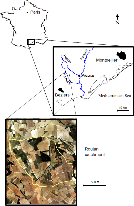
Vineyards cover about 60% of the area of this basin, divided into more than 230 field entities (Moussa et al., 2002), mainly vineyards gobelets, chemically weeded, or vineyards palissees, weeded by soil tillage and with wider ranks. Young vineyards (plantiers) are organized as palissees, which is a more recent technique. The man-made ditch network follows the plot margins and has a total length of 11,069 m. At the Roujan catchment there are no natural ditches and they are of variable density and size. Surface elevation of the catchment ranges from 76 to 128 m with slopes between 2 and 18%.
The climate is Mediterranean with a long dry season and an average annual temperature of 14.2°C. Annual rainfall varies between 500 and 1400 mm (MOUSSA et al., 2002) with a mean of 650 mm (HÉBRARD et al., 2006). Precipitations occur essentially in the form of brief and intense storms in spring or autumn and result in predominant Hortonian runoff associated with short response-times throughout the basin. Enhanced by pedo-climatic conditions, overland flow indeed explains 80% of the peak discharge (MOUSSA et al., 2002). The runoff coefficient for the entire basin varies from 0 to 68% in the first 30 to 60 minutes after rainfall is initiated (MOUSSA et al., 2002) and runoff volume was estimated to be about 70% of the rain volume on a non-tilled plot. Ditches play a major role in guiding the flow towards the outlet. Though event-dominated, the hydrological behaviour of the basin has seasonal characteristics. Three hydrological periods appear: (i) high watertable levels from October to May, with ditch drainage and permanent baseflow that becomes strong during rain events; (ii) lowest watertable levels during summer months, with no baseflow and intense but rare rainfall events that do not affect the outlet flow because of infiltration in plots and ditches and (iii) high watertable levels at the beginning of autumn, with intense and frequent rainfall events that quickly and totally recharge groundwaters units.
2.1.1 The measurement devices
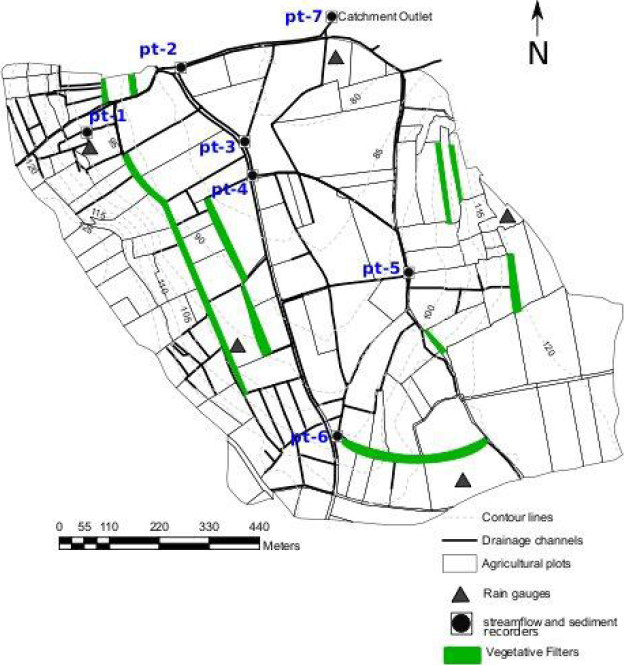
The catchment has been instrumented with hydro-meteorological equipment since 1992 (meteorological station, rain gauges, streamflow recorders, piezometers, tensio-neutronic sites, automatic sediment samplers, Venturi channels). Figure 2 shows the localization of some measurement devices.
Figure 2
Meteo-hydro-sedimentological devices in the Roujan agricultural catchment.
Équipement hydrométéorologique et échantillonneurs automatiques installés à Roujan.
The funnel rain gauge system allows recording every 5 min. The outflow is measured from depth gauges set up in Venturi channels and is recorded every 5 min or every 10 min if the variation in height between two recordings is less than 10 mm. Measurement of the quantity of suspended material is done with an automatic sampling apparatus collecting small liquid volumes at determined water height, immediately upstream of the Venturi channel. The choice of water heights used in collecting particle-laden water is a function of the drainage area and its observed hydrological behaviour. The samplings continue with one sampling every 30 mm variation during the flood phase and then during the decrease of water height.
Global sampling systems put each sample in the same recipient to form an average concentration in suspended materials during an event. Sequential sampling systems put each sample in a separate recipient to monitor the evolution of the instantaneous concentration during the event. The samples are passed through 0.45 μm filters, the filters are then dried at 105°C for 48 h and finally weighed in order to get the mass concentration of suspended materials.
2.2 Rainfall events
After statistical analyses of rainfall events over the 2005-2007 period, 10 rainfall events were chosen for calibration and validation procedures. They vary in duration from 2 h 10 min to 1 day 16 h 10 min, for total rainfall amounts varying from 20 mm to 92 mm. Sub-catchments and catchment lag times are short, generally less than 30 min. Table 1 shows the principal characteristics of these selected rainfall events.
Table 1
Main rainfall characteristics for calibration and validation events, Ca corresponds to calibration events, Imean, the mean rainfall intensity, Imax, the maximum rainfall intensity and IPA5, an index of antecedent rainfall events.
Caractéristiques des événements pluvieux utilisés pour le calage et la validation du modèle, Ca correspond aux événements de calage, Imean, l’intensité moyenne, Imax, l’intensité maximum de la pluie, IPA5, l’indice de précipitation précédente sur 5 jours.

We performed a PCA (Principal Component Analysis) using as factors the total amount of rain, the maximum intensity and the effective duration of rainfall. The PCA analysis was performed with R software (R core team 2013). Seven calibration rainfall events were chosen (2007-06-10, 2007-06-06, 2006-10-18, 2006-01-15, 2005-11-12, 2005-10-18) and the four remaining events (2007-03-31, 2006-09-13, 2006-10-11, 2007-02-17) were used in validation procedures. The eingenvalues displayed in the histogramm of the left upper corner of Figure 3 demontrate that more than 80% of the variance is explained by the first and second components; this validates the PCA. From the PCA analysis (Figure 3) we observed that two of the eleven rainfall events are positioned as outliers.
Figure 3
Principal component analysis of the eleven rainfall events where: IPA5 is the five day anterior rainfall; duration, the time from rainfall beginning to the end of event; Imax, the maximum rainfall intensity during the event; the x axis, the first component and the y axis, the second component.
Analyse en composantes principales (ACP) : IPA5, indice de précipitation précédente sur cinq jours; duration, la durée de l’événement pluvieux; Imax, l’intensité maximale de l’événement pluvieux; l’axe des x, la première composante, et l’axe des y, la deuxième composante.

It can be seen from Figure 3 that rainfall events 2005-11-12 (6) and 2006-10-11 (9) are outliers. The 2005-11-12 rainfall event has the longest duration and rainfall amount and the 2006-10-11 event has the highest maximum intensity. Both 2005-11-12 and 2006-10-11 are different from the other rainfall events.
2.3 Model description
The MHYDAS-Erosion model has been developed under the OpenFLUID software development environment as a module of the hydrological MHYDAS model (MOUSSA et al., 2002). The catchment is subdivided into homogeneous hydrological units labelled ‘SUs’ for ‘surface units’ and ‘RSs’ for ‘reach segments’. These two constitutive elements were found to be necessary to take into account the variability and discontinuities of the agricultural catchments in a procedure extensively described by MOUSSA et al. (2002). SUs are polygons that represent areas (e.g. agricultural plots), whereas RSs are lines that represent concentrated flow (e.g. drainage channels and rivers). Where information is available, RSs may be determined by field observation and aerial photography. Otherwise, RSs are determined using the classic flow accumulation procedures included in the GeoMHYDAS software (LAGACHERIE et al., 2010) or other geographical information system (GIS) tools.
At the SU level, rain is partitioned between infiltration and runoff according to the method of MOREL-SEYTOUX (1978). Available runoff is thus derived from rain characteristics, saturated vertical hydraulic conductivity and initial water content. The one-dimensional Saint Venant equations are then solved through a specific analytical method (MOUSSA and BOCQUILLON, 1996) for runoff transfer. Flow depth and velocity for concentrated flows in linear reach elements are then obtained from the discharge partition with the Manning formula by assuming the slope, shape and width of each reach segment are known. As in WEPP (LAFLEN et al., 1997), the erosion module enables a finer decomposition of SUs into sub-elements of adaptable sizes representing rill and interrill areas associated with specific phenomenologies. To ensure the stability of the model according to the Courant-Friedrichs-Lewy (CFL) condition (COURANT et al., 1928), we use a time step fine enough to correctly track the highest possible flow velocities. The parameterization and use of MHYDAS-Erosion are guided by the available GIS vector-based environment. To be able to integrate the spatial and temporal impacts of Best Management Practices (BMPs) on water-sediment pathways and transport, a specific connectivity module has been developed in MHYDAS-Erosion.
MHYDAS-Erosion is based on the mass conservation principle applied to sediment load proposed by BENNETT (1974):
where h (m) is the water height, c (kg•m‑3) is the sediment concentration, t (s) is time, U (m•s‑1) is the mean flow velocity, Di (kg•m‑2•s‑1) is the sediment inflow rate due to interrill erosion, Dr (kg•m‑2•s‑1) is the sediment inflow rate due to rill erosion and Dd (kg•m‑2•s‑1) is the sediment deposition rate, which eventually coexists with Dr. MHYDAS-Erosion only takes into account suspended load sediment transport.
The sediment inflow rate due to interrill erosion Di can be calculated using two different equations, one is based on the soil aggregate stability and the other one is based on splash cup measurements (for more details, see GUMIERE et al., 2011). For this work we have chosen to use Eq. (2) which is based on the aggregate stability.
where As is the index of stability calculated from mean weight diameter (MWD) measurements (YAN et al., 2008), I (mm•h‑1) is the rainfall intensity and Sfactor (-) is the slope factor calculated by (1.05-0.85•e-4sinθ) where θ is the slope angle. In MHYDAS-Erosion, we consider that the water height on interrill areas is too shallow to apply the transport equations used in conventional hydraulics. The concept of CETI (efficiency in transport on interrills) was introduced to describe the effect of the perpendicular roughness on the interrill-to-rill erosion contribution. Its values are calculated with , where CETImax (-) is the maximum allowed value of CETI, α (-) is an empirical exponent depending on roughness and R (mm•h‑1) is the runoff amount.
The sediment inflow rates due to rill erosion Dr, integrate two aspects into a single equation. When the transport capacity of the flow exceeds the current sediment load, both particle detachment due to excess shear stress exerted by the flow and sediment transport appear in the Eq. (3) proposed by FOSTER et al. (1995):
where kr (s•m‑1) is rill erodibility, τ (Pa) is the shear stress exerted on the bed by the flow, τc (Pa) is the critical shear stress over which detachment is initiated, qs (kg•m‑1•s‑1) is the unit solid discharge by a 1 m width of the flow calculated as qs = q•c and TC (kg•m‑1•s‑1) is transport capacity, which measures the ability of the flow to carry a sediment load.
Sediment deposition Dd is calculated with Eq. (4), under the qs > TC condition (FOSTER et al., 1995)
where vs (m•s‑1) is the settling velocity calculated with the equation proposed by SOULSBY (1997).
The hydrological and erosion equations are solved independently but successively within the same time step of a priori fixed duration. Sediment mass balance equation (Eq. (1)) is solved at each time step using a backward explicit finite difference scheme. Table 2 shows the input parameters required to run MHYDAS-Erosion. They have specific values for each hydrological object (SU or RS).
Table 2
Input parameters necessary to run MHYDAS-Erosion.
Paramètres d’entrées pour le MHYDAS-Erosion.

2.4 Model calibration and validation procedure
2.4.1 Calibration parameters
In order to avoid or at least diminish equifinality (BRAZIER et al., 2000), we reduced the number of calibration parameters, based on previous sensitivity analyses of the model (CHEVIRON et al., 2010 and 2011). Considering the dependence of erosion processes on hydrological processes, we calibrated hydrology first and then erosion. In fact, in MHYDAS-Erosion, as well as in most erosion models, erosion variables are calculated using previously calculated hydrological variables. The influence of error from hydrological output has been pointed out by WAINWRIGHT and PARSONS (1998), who demonstrated that correct determination of flow depth was critical for erosion estimations. The flow depth at any location will depend on the prediction of infiltration rate, resistance to flow and flow routing, causing hyper-sensibility of modelled erosion processes to the previously calculated hydrological outputs. We have thus chosen to calibrate hydrological outputs at best, to avoid transmitting hydrological errors to the erosion module. We may thus better identify errors specific to the erosion module.
For the calibration procedure, we chose the saturated hydraulic conductivity Ks, which is the most sensitive hydrological parameter in the MHYDAS-Erosion model. Values of Ks were divided into four classes attributed to the hydrological units according to reported land uses. To prevent equifinality, each class value for Ks is linked to the reference value Ks1: Ks2 = 2Ks1, Ks3 = 3Ks1. The given initial values for each Ks class related to a given land use are Ks0 = 5.5E-9 m•s‑1 for roads and impermeable surfaces, Ks1 = 5.5E-7 m•s‑1 for tillage vineyards, Ks2 = 1.1E-7 m•s‑1 for non-tillage vineyards and annual crops and Ks3 = 2.2E-6 m•s‑1 for forests, fallows and scrublands. MHYDAS-Erosion uses an equivalent infiltrability parameter defined as Ce for infiltration in the ditch network. It describes transfers between ditches and groundwater units. The reference value adopted to Ce is 1.2E-3 m•s‑1.
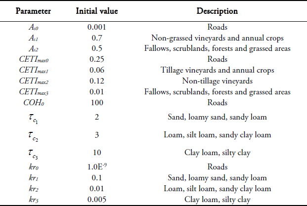
Erosion parameters chosen for calibration were the index of stability (As), rill erodibility (kr), soil critical shear stress and the maximum value of the coefficient for efficiency of interrill transport (CETImax). Initial (i.e. starting) values used in calibration of erosion parameters were obtained from land use reports (Table 3). In the Roujan catchment the ditches are man-made and for this work we have considered them to be homogeneous; initial values of and were fixed for all ditches in the catchment. Note that since the critical shear stress is highly related to soil cohesion, COH (Pa), the former was approximated by the latter in the downstream direction. The time step used for the calibration procedure was 1 min. The catchment was subdivied into 223 SUs and 159 RSs.
Table 3
Calibration parameters for erosion processes.
Paramètres de calage.
2.4.2 Automatic calibration procedure with PEST
We used PEST software (DOHERTY, 2004) to calibrate parameter sets for MHYDAS-Erosion. PEST is a non-linear parameter estimation software that uses the Gauss-Marquardt-Levenberg (MARQUARDT, 1963) algorithm with an iterative process. At the beginning of each iteration the relationship between model parameters and model-generated observations is linearised by formulating it as a Taylor expansion around the current best parameter set, and hence the derivatives of all observations with respect to all parameters must be calculated. This linearised problem is then solved for a better parameter set, and the new parameters are tested by running the model again, under user-defined options. By comparing parameter changes and objective function improvement achieved through the current iteration with those achieved in previous iterations, PEST can tell whether it is worth undertaking another optimisation iteration, if so the whole process is repeated. It acts as a master model to any slave model to which it is linked, provided the communication between them is possible through input and output ASCII files (Figure 4).
Figure 4
Calibration scheme proposing a coupling between MHYDAS-Erosion, PEST, and auxiliary programs involved in post-treatments.
Schéma de calage, couplage entre MHYDAS-Erosion, PEST et les programmes auxiliaires.

The calibration procedure is performed in two steps. It starts with the calibration of the total flow discharge from the agricultural field scale, i.e. over the entire basin. In fact, the agricultural field scale is a kind of "learning stage" where the optimum value of Ks1 is obtained for a specific land use. We then relied on literature and expert opinion to determine the multiplicative factors between the different Ks values corresponding to different land uses. In this case study, Ks1 corresponds to vineyards with chemical tillage that favours crusting formation and decreases infiltrability (Le Bissonnais and Singer, 1992). The Ks2 = 1.1Ks1 values corresponds to vineyards with mechanical tillage or to annual crops, which favour infiltration. The Ks3 = 1.7Ks1 corresponds to forests and natural vegetation. In the second step, the multi-scale calibration is applied using the seven measurement points over the Roujan catchment. The multi-scale calibration procedure consists of fixing the Ks values obtained during the first step and varying Ce values. The aim is to reach the minimum difference between observed and simulated flow discharge for each measurement point simultaneously.
Erosion parameters were calibrated the same way, using the agricultural field scale as a "learning stage". Values of As1, CETImax1, and kr1 were first calibrated with total soil loss values at the agricultural field scale, and then multiplying factors were introduced with reference to known land uses. At the end of the calibration procedures, a set of erosion parameters was defined. Validation procedures adopted in this case study consisted of identifying an average parameter set for the seven calibration events. The model was then run for the four validation events with the average parameter set: total soil loss simulated for each rainfall event at each measurement point was compared with observed values. The statistical evaluation criteria used in this work were the root mean square error (RMSE), the ratio of RMSE to the standard deviation of the observations (RSR), the modified Nash-Sutcliffe efficiency (mNSE), the index of agreement (d), the coefficient of determination (R2). These criteria were chosen because they reflect different evaluation properties of the model (DAWSON et al., 2007). Table 4 shows the statistical evaluation criteria and their respective ranges.
Table 4
Evaluation criteria and their respective ranges; Yi is the observed value,  i the simulated value, n, the sample size and
  i, the mean of the observed values.
Critères d’évaluation du modèle et leurs intervalles respectifs; Yi est la valeur observée,  i, la valeur simulée, n, le nombre de points et
  i, la moyenne des valeurs observées.

3. Results and Discussion
In Table 5, where calibrated values of the hydrological and erosion parameters for the ten rainfall events are shown, it can be observed that Ks1 values have a coefficient of variation (CV) of 1.05. These values are coherent with those found in other studies in the Roujan catchment (CHAHINIAN et al., 2006a, 2006b; MOUSSA et al., 2002). The coefficient of variation of Ce values is 2.03. We calibrated Ks and Ce for all rainfall events because of the high sensitivity of the model to these parameters (CHEVIRON et al., 2010), which also have a high spatial variability (GUMIERE et al., 2007). As shown by the coefficients of variation, the widest adjustments were made on Ce, showing a higher dependence of MHYDAS-Erosion on this parameter than on Ks. Another possible explanation is that starting Ce values were less precisely chosen than the Ks values.
Table 5
Hydrological and erosion calibrated input parameters.
Valeurs des paramètres hydrologiques et d’érosion après la procédure de calage.

Concerning the erosion parameters, only CETImax, krRS and τcRS had their values adjusted during the seven calibration events. Calibrated values for erosion parameters are shown in Table 5. It can be observed that CETImax has a variation coefficient of 0.61. Values of krRS have a variation coefficient of 1.81, and values of τcRS have a variation coefficient of 1.81. Though freely adjustable, parameters As, τcSU and kr remained at their reference value. From the coefficients of variation, rill erodibility in linear elements (krRS) was the most affected parameter.
Results for calibration of total dischage and total soil loss simulated with MHYDAS-Erosion for the Roujan catchment are presented in Figure 5.
Figure 5
Calibration results for total discharge and total soil loss, (a scatter plot of simulated and observed total discharge, (b) box-plot of the difference between the simulated and the observed values of discharge for all observation points in the Roujan catchment, (c) scatter plot of simulated and observed total soil loss, (d) box-plot of the difference between the simulated and the observed values of soil loss for all observation points.
Résultats du calage, débit total et pertes en sols, (a) diagramme de dispersion entre les valeurs simulées et observées de débit total, (b) box-plot des différences entre les valeurs simulées et observées des débits à tous les points de mesures du bassin versant. (c) diagramme de dispersion entre les valeurs simulées et observées de perte en sols, (d) box-plot des différences entre les valeurs simulées et observées des pertes en sols à tous les points de mesures du bassin versant.
a

b

c
d

Figure 5a presents a scatter plot between the simulated and observed values of total discharge for the seven observation points and the 10 rainfall events, in the Roujan catchment (cf. Figure 2). The points in the figure are close to the 1:1 line, indicating a good (R2 = 0.95) agreement between simulated and observed values. Dispersion observed in Figure 5a is associated with the worst simulation points, whereas most data are grouped near 0 to 50 m3•ha‑1. Values of total discharge indicated that (at least) for these rainfall events, Roujan catchment has a low-to-moderate runoff coefficient (ranging from 1.0 to 10%).
Figure 5b shows the boxplot for the absolute error between the simulated and the oberved total discharge values of each measurement point. The maximum value of the difference between observed and simulated flow discharges is 132 m3•ha‑1. It was obtained at point 5 (sub-catchment scale) for the strongest rainfall event (2005-11-12). The minimum value of the difference is 0.00 m3•ha‑1 points 1 and 7 (agricultural field and outlet catchment scale). In fact, the dispersion error is mostly due to a few events that are not simulated well, such as that of 2005-11-12. This rainfall event is the longest in the dataset (1810 min, about 1.6 days) and because the event-based characteristic of MHYDAS-Erosion, the model has difficulty in simulating long rainfall events. These events are often associated with non-Hortonian runoff processes, such as subsurface runoff and exfiltration processes, which are not taken into account in MHYDAS-Erosion. Previous studies at the Roujan catchment have shown that exfiltration may represent up to 100% of total discharge at the outlet catchment (CHAHINIAN, 2004) under certain circumstances.
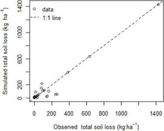
Figure 5c presents a scatter plot between the simulated and observed values of total soil loss for the seven observation points and the six calibration rainfall events (cf. Table 1), in the Roujan catchment. Figure 5c shows a very good agreement between simulated and observed values (R2 = 0.97). Dispersion observed in Figure 5c is associated with the worst simulation points, whereas most data are grouped near 0 to 200 kg•ha‑1. If we may suppose that five erosive rainfall events (producing 200 kg•ha‑1) occur per year in the Roujan catchment, this would give a rate of annual erosion of 1 ton•ha‑1•year‑1, which is very low compared with other world regions.
Figure 5d presents the boxplot for the absolute error between simulated and observed total soil loss values for each measurement point. The maximum value of the difference between observed and simulated flow discharges is 206 kg•ha‑1. It was obtained at point 5 (sub-catchment scale) for the strongest rainfall event (2005-11-12), as in the hydrology results. This result indicates that poor results in the hydrology module of MHYDAS-Erosion may drive poor results in the erosion module. Meanwhile, differences of about 20-30% in rainfall amount have been recorded among the five rain gauges distributed over the catchment. Moreover, the exfiltration phenomenon may also affect soil loss values. The minimum value of the difference is 0.00 m3•ha‑1 at points 1, 3 and 7 (agricultural field, sub-catchment and outlet catchment scale).
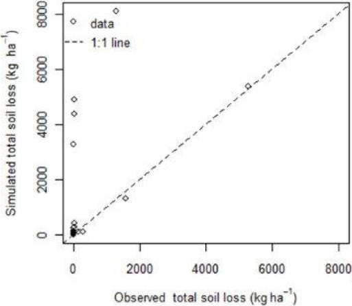
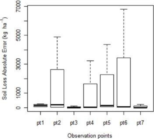
Figure 6a presents a scatter plot between the simulated and observed values of total soil loss for the seven observation points and the four validation rainfall events (cf. Table 1). Figure 6a shows poor agreement between simulated and observed values (R2 = 0.25). Figure 6b shows that total soil loss has been simulated within an average difference of 766 kg•ha‑1, all scales considered. The maximum value of the difference between observed and simulated soil loss is 6794 kg•ha‑1, at the point 6 (sub-catchment scale) for the event 2006-10-11. The minimum value of the difference is 0.00 kg•ha‑1, often found at points 1, 3 and 7 (agricultural field, sub-catchment and outlet catchment scale). Most of the data dispersion is caused by rainfall event 9 (2006-10-11). In fact, rainfall event 9 is an average rainfall event with a very low observed soil loss in comparison with other average rainfall events. Table 1 indicates the highest Imax (124 mm•h‑1), which is approximately 4 times the average Imax when considering all rainfall events. MHYDAS-Erosion highly overstimates the interrill erosion for this rainfall event. We suspect that the rainfall intensity of rainfall event 9 exceeds the calibration range of equation 2, proposed by Yan et al. (2008) (interill erosion Di and the CETI equation).
Figure 6
Validation results for total soil loss, (a) scatter plot of simulated and observed total soil loss for the four validation events, (b) box-plot of the difference between the simulated and the observed values of soil loss for all observation points in the Roujan catchment, (c) scatter plot of simulated and observed total soil loss without event 9, (d) box-plot of the difference between the simulated and the observed values of soil loss for all observation points without event 9.
Résultats de la validation, débit total et pertes en sols, (a) diagramme de dispersion entre les valeurs simulées et observées de débit total, (b) box-plot des différences entre les valeurs simulées et observées des débits à tous les points de mesures du bassin versant. (c) diagramme de dispersion entre les valeurs simulées et observées des pertes en sols, (d) box-plot des différences entre les valeurs simulées et observées des pertes en sols à tous les points de mesures du bassin versant.
a
b
c

d
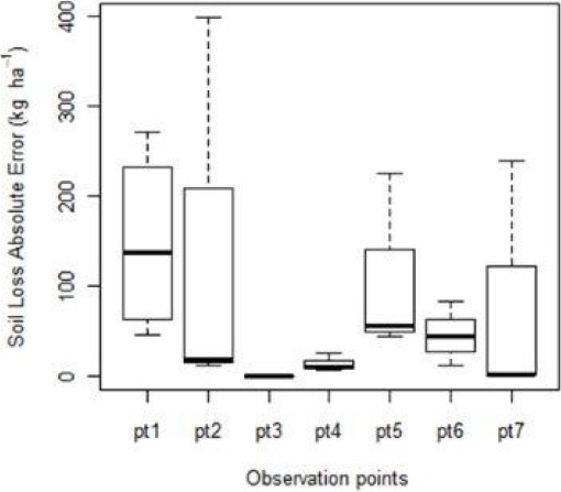
Figure 6c presents a scatter plot between the simulated and observed values of total soil loss for the seven observation points and the validation events, without event 9. Without event 9, Figure 6c shows a very good agreement between simulated and observed values (R2 = 0.96). Also the highest difference between simulated and observed soil loss has dropped, from 6794 to 400 kg•ha‑1 without event 9. This result indicates that for a high intensity rainfall event, MHYDAS-Erosion may highly overestimate soil loss. Table 6 summaries the overall model efficiency criteria for both calibration and validation events.
Table 6
Summary of global model efficiency
Performance globale du modèle

Discrepancies between observed and simulated values are generally higher at measurement points associated with sub-catchment scales, where the hydrological error is somehow transmitted into erosion modelling.
4. Conclusion
In this work we have presented a case study of the multi-scale calibration and validation of the MHYDAS-Erosion model for a Mediterrnean vineyard catchment. We used spatially-distributed data of soil loss and runoff, collected for seven entities at three different scales in the Roujan catchment. We have associated expert knowledge in linking physical parameters to land uses with the automatic calibration software PEST. Acceptable results were obtained in terms of parameter values, identification of their physical meaning and coherence. However, some limitations have been identified too, which could be remedied in more detailed studies involving (i) spatially-distributed rainfall on the catchment, (ii) a description of groundwater exfiltration and (iii) spatially-distributed properties of the ditches over the catchment. Nevertheless, a richer parameterisation would reactivate the risk of equifinality unless precise information is available.
A large difference between observed and simulated total soil loss values was observed for two of the ten rainfall events (events 6 and 9). For these rainfall events the model over predicted total soil loss for all catchment measurement points, except for the plot scale (point 1). This result, related to event 9, could be an overestimation of the interrill detachment rate simulated by the model. Regarding event 6, a possible explanation may be that MHYDAS-Erosion does not have a good representation of non-Hortonian runoff production.
In fact, more studies may be done with these kind of rainfall events to understand model behaviour. However, hydrological and erosive phenomena were simulated with acceptable precision at the three intricate scales accounting for the catchment, sub-catchment and plot scales. It is important to note that calibration and validation may respect the principle of unity of place (DE MARSILY, 1994). The application of MHYDAS-Erosion to another catchment would certainly need specific calibration.
Appendices
Ackowledgments
We are grateful to the two anonymous reviewers for providing useful comments to improve the quality of the manuscript. We also thank the ANR (National Research Agency) for funding of the MESOEROS project. The first author thanks the support of the National Council of Technological and Scientific Development of Brazil (CNPQ-Brazil).
Bibliographical References
- BEVEN K.J. (1989). Changing ideas in hydrology: the case of physically based models. Hydrol. J., 105, 157-172.
- BENNETT J.P. (1974). Concepts of mathematical modeling of sediment yield. Water Resour. Res., 10, 485-492.
- BOARDMAN J. (2006). Soil erosion science: Reflections on the limitations of current approaches. Catena, 68, 73-86.
- BRAZIER R.E., K.J.BEVEN, J. FREER and J.S. ROWAN (2000). Equifinality and uncertainty in physically based soil erosion models: application of the glue methodology to wepp-the water erosion prediction project – for sites in the UK and USA. Earth Surf. Proc. Landforms, 25, 825-845.
- CHAHINIAN N.(2004). Paramétrisation multicritère et multiéchelle d’un modèle hydrologique spatialisé de crue en milieu agricole. Thèse de Doctorat, Université de Montpellier II, France, 323 p.
- CHAHINIAN N., R. MOUSSA, P. ANDRIEUX and M. VOLTZ (2006a). Accounting for temporal variation in soil hydrological properties when simulating surface runoff on tilled plots. J. Hydrol., 326, 135-15.
- CHAHINIAN N., M. VOLTZ, R. MOUSSA and G. TROTOUX (2006b). Assessing the impact of the hydraulic conductivity of a crusted soil on overland flow modelling at the field scale. Hydrol. Proc., 20, 1701-172.
- CHEVIRON B., S.J. GUMIERE, Y. LE BISSONNAIS, D. RACLOT and R. MOUSSA (2010). Sensitivity analysis of distributed erosion models - framework. Water Resour. Res., 46, W08508.
- CHEVIRON B., Y. LE BISSONNAIS, J.-F. DESPRATS, A. COUTURIER, S.J. GUMIERE, O. CERDAN, F. DARBOUX and D. RACLOT (2011). Comparative sensitivity analysis of four distributed erosion models, Water Resour. Res., 47, W01510.
- CITEAU L., A.M. BISPO, M. BARDY and D. KING (2008). Gestion durable des sols. QUAE RENAUD-BRAY (Éditeur), Versailles, 320 p.
- COURANT R., K. FRIEDRICHS and H. LEWY(1928). Über die partiellen differenzengleichungen der mathematischen physik. Math. Annal.,en 100, 32-74.
- DAWSON C., R. ABRAHART and L. SEE (2007). Hydrotest: a web-based toolbox of evaluation metrics for the standardised assessment of hydrological forecasts. Environ. Model. Software, 22, 1034-1052.
- DE MARSILY G.(1994). On the use of models in hydrology [Free opinion] - De l’usage des modèles en hydrologie [Tribune libre]. Rev. Sci. Eau, 7, 219-234.
- DE ROO A.P.J. and V.G. JETTEN (1999). Calibrating and validating the LISEM model for two data sets from the Netherlands and South Africa. Catena, 37, 477-493.
- DE VENTE J. and J. POESEN (2005). Predicting soil erosion and sediment yield at the basin scale: Scale issues and semi-quantitative models. Earth Sci. Rev., 71, 95-125.
- DOHERTY J. (2004). PEST - Model-independent parameter estimation, User Manual. Watermark Numerical Computing.
- FOSTER G.R., D.C. FLANAGAN, M.A. NEARING, L.J. LANE, L.M. RISSE and S.C. FINKNER (1995). Water erosion prediction project (WEPP): technical documentation. Tech. report. NSERL Report No. 10. National Soil Erosion Research Laboratory. USDA-ARS-MWA. 1196 Soil Building, West Lafayette, NO, USA, 47, 907-1196.
- GUMIERE S.J., M. MORAES and R.L. VICTORIA (2007). Calibration and validations of a soil-plant-atmosphere model at the national forest of tapajós, pará. Braz. J. Water Res., 1, 1-11.
- GUMIERE S.J., D. RACLOT, B. CHEVIRON, G. DAVY, X. LOUCHART, J.-C. FABRE, R. MOUSSA and Y.L. BISSONNAIS (2011). MHYDAS-erosion: a distributed single-storm water erosion model for agricultural catchments. Hydrol. Process., 25, 1717-1728.
- HÉBRARD O., M. VOLTZ, P. ANDRIEUX and R. MOUSSA (2006). Spatio-temporal distribution of soil surface moisture in a heterogeneously farmed Mediterranean catchment. J. Hydrol., 329, 110-121.
- HESSEL R., R. VAN DEN BOSCH and O. VIGIAK (2006). Evaluation of the LISEM soil erosion model in two catchments in the East African highlands. Earth Surf. Proc. Landforms, 31, 469-486.
- JETTEN V.G., A.P.J. DE ROO and D. FAVIS-MORTLOCK (1999). Evaluation of field-scale and catchment-scale soil erosion models. Catena, 3, 521-541.
- KLIMENT Z., J. KADLEC and J. LANGHAMMER (2008). Evaluation of suspended load changes using ANNAGNPS and SWAT semi-empirical erosion models. Catena, 73, 286-299.
- LAFLEN J.M., W.J. ELLIOT, D.C. FLANAGAN, C.R. MEYER and M.A. NEARING (1997). Wepp-predicting water erosion using a process-based model. J. Soil Water Conserv., 52, 96-102.
- LAGACHERIE P., M. RABOTIN, F. COLIN, R. MOUSSA and M. VOLTZ (2010). Geo-MHYDAS: a landscape discretization tool for distributed hydrological modeling of cultivated areas. Comput. Geosci., 36, 1021-1032, DOI: 10.1016/j.cageo.2009.12.005.
- LE BISSONNAIS Y., C. MONTIER, J. JAMAGNE, J. DAROUSSIN and D. KING (2002). Mapping erosion risk for cultivated soil in France. Catena, 46, 207-220.
- LE BISSONNAIS Y. and M. SINGER (1992). Crusting, runoff and erosion response to soil water content and successive rainfall events. Soil Sci. Soc. Am. J., 56, 1898-1903.
- MARQUARDT D.W.(1963). An algorithm for least-squares estimation of non-linear parameters. J. Soc. Ind. Appl. Math., 11, 431-441.
- MOREL-SEYTOUX H.J. (1978). Derivation of equations for variable rainfall infiltration. Water Resour. Res., 14, 561-568.
- MORGAN R.P.C. (2001). A simple approach to soil loss prediction: a revised Morgan-Morgan-Finney model. Catena, 44, 305-322.
- MOUSSA R. and C. BOCQUILLON (1996). Algorithms for solving the diffusive wave flood routing equation. Hydrol. Proc., 10, 105-124.
- MOUSSA R., M. VOLTZ and P. ANDRIEUX (2002). Effects of the spatial organization of agricultural management on the hydrological behaviour of a farmed catchment during flood events. Hydrol. Proc., 16, 393-412.
- NEARING M.A. (2000). Evaluating soil erosion models using measured plot data: accounting for variability in the data. Earth Surf. Proc. Landforms, 25, 1035-1043.
- R CORE TEAM (2013). R: A language and environment for statistical computing. R Foundation for Statistical Computing, Vienna, Austria. URL http://www.R-project.org/, (consulted in March 2013).
- SOULSBY R.L. (1997). Dynamics of marine sands: A manual for practical applications. Thomas Telford (Editor), London, UK, 250 p.
- TAKKEN I., L. BEUSELINCK, J. NACHTERGAELE, G. GOVERS, J. POESEN and G. DEGRAER (1999). Spatial evaluation of a physically-based distributed erosion model (LISEM). Catena, 37, 431-447.
- WAINWRIGHT J. and A. J. PARSONS (1998). Modelling soil erosion by water. In: Sensitivity of sediment-transport equations to errors in hydraulic models of overland flow,Springer-Verlag (Editor), Berlin, pp. 271-284.
- YAN F.-L., Z.H. SHI, Z.X. LI and C.F. CAI (2008). Estimating interrill soil erosion from aggregate stability of ultisols in subtropical China. Soil Till. Res., 100, 34-41.
List of figures
Figure 1
Roujan catchment, France.
Le bassin versant de Roujan, France.
Figure 2
Meteo-hydro-sedimentological devices in the Roujan agricultural catchment.
Équipement hydrométéorologique et échantillonneurs automatiques installés à Roujan.
Figure 3
Principal component analysis of the eleven rainfall events where: IPA5 is the five day anterior rainfall; duration, the time from rainfall beginning to the end of event; Imax, the maximum rainfall intensity during the event; the x axis, the first component and the y axis, the second component.
Analyse en composantes principales (ACP) : IPA5, indice de précipitation précédente sur cinq jours; duration, la durée de l’événement pluvieux; Imax, l’intensité maximale de l’événement pluvieux; l’axe des x, la première composante, et l’axe des y, la deuxième composante.
Figure 4
Calibration scheme proposing a coupling between MHYDAS-Erosion, PEST, and auxiliary programs involved in post-treatments.
Schéma de calage, couplage entre MHYDAS-Erosion, PEST et les programmes auxiliaires.
Figure 5
Calibration results for total discharge and total soil loss, (a scatter plot of simulated and observed total discharge, (b) box-plot of the difference between the simulated and the observed values of discharge for all observation points in the Roujan catchment, (c) scatter plot of simulated and observed total soil loss, (d) box-plot of the difference between the simulated and the observed values of soil loss for all observation points.
Résultats du calage, débit total et pertes en sols, (a) diagramme de dispersion entre les valeurs simulées et observées de débit total, (b) box-plot des différences entre les valeurs simulées et observées des débits à tous les points de mesures du bassin versant. (c) diagramme de dispersion entre les valeurs simulées et observées de perte en sols, (d) box-plot des différences entre les valeurs simulées et observées des pertes en sols à tous les points de mesures du bassin versant.
a
b
c
d
Figure 6
Validation results for total soil loss, (a) scatter plot of simulated and observed total soil loss for the four validation events, (b) box-plot of the difference between the simulated and the observed values of soil loss for all observation points in the Roujan catchment, (c) scatter plot of simulated and observed total soil loss without event 9, (d) box-plot of the difference between the simulated and the observed values of soil loss for all observation points without event 9.
Résultats de la validation, débit total et pertes en sols, (a) diagramme de dispersion entre les valeurs simulées et observées de débit total, (b) box-plot des différences entre les valeurs simulées et observées des débits à tous les points de mesures du bassin versant. (c) diagramme de dispersion entre les valeurs simulées et observées des pertes en sols, (d) box-plot des différences entre les valeurs simulées et observées des pertes en sols à tous les points de mesures du bassin versant.
a
b
c
d
List of tables
Table 1
Main rainfall characteristics for calibration and validation events, Ca corresponds to calibration events, Imean, the mean rainfall intensity, Imax, the maximum rainfall intensity and IPA5, an index of antecedent rainfall events.
Caractéristiques des événements pluvieux utilisés pour le calage et la validation du modèle, Ca correspond aux événements de calage, Imean, l’intensité moyenne, Imax, l’intensité maximum de la pluie, IPA5, l’indice de précipitation précédente sur 5 jours.
Table 2
Input parameters necessary to run MHYDAS-Erosion.
Paramètres d’entrées pour le MHYDAS-Erosion.
Table 3
Calibration parameters for erosion processes.
Paramètres de calage.
Table 4
Evaluation criteria and their respective ranges; Yi is the observed value, i the simulated value, n, the sample size and i, the mean of the observed values.
Critères d’évaluation du modèle et leurs intervalles respectifs; Yi est la valeur observée, i, la valeur simulée, n, le nombre de points et i, la moyenne des valeurs observées.
Table 5
Hydrological and erosion calibrated input parameters.
Valeurs des paramètres hydrologiques et d’érosion après la procédure de calage.
Table 6
Summary of global model efficiency
Performance globale du modèle