

Résumés
Abstract
Parameter estimation and model fitting underlie many statistical procedures. Whether the objective is to examine central tendency or the slope of a regression line, an estimation method must be used. Likelihood is the basis for parameter estimation, for determining the best relative fit among several statistical models, and for significance testing. In this review, the concept of Likelihood is explained and applied computation examples are given. The examples provided serve to illustrate how likelihood is relevant, and related to, the most frequently applied test statistics (Student’s t-test, ANOVA). Additional examples illustrate the computation of Likelihood(s) using common population model assumptions (e.g., normality) and alternative assumptions for cases where data are non-normal. To further describe the interconnectedness of Likelihood and the Likelihood Ratio with modern test statistics, the relationship between Likelihood, Least Squares Modeling, and Bayesian Inference are discussed. Finally, the advantages and limitations of Likelihood methods are listed, alternatives to Likelihood are briefly reviewed, and R code to compute each of the examples in the text is provided.
Keywords:
- parameter estimation,
- modeling Likelihood,
- Likelihood ratio,
- R script
Résumé
L’estimation de paramètres et l’ajustement de modèles est au coeur de toutes procédures statistiques. Que l’objectif soit d’examiner la tendance centrale ou une pente de régression, une méthode d’estimation est nécessaire. La fonction de vraisemblance est la pierre angulaire sur laquelle repose l’estimation de paramètres, les tests d’hypothèses et la comparaison de modèles. Cet article présente le concept de vraisemblance et les tests statistiques communément utilisés (tests t, ANOVA). Certains exemples présentent le calcul de la fonction de vraisemblance lorsque le postulat de normalité est présent et lorsqu’il n’est pas adéquat. Les liens entre vraisemblance, rapport de vraisemblance, méthodes des moindres carrés et bayésienne sont discutés. Finalement, les forces et les faiblesses des méthodes basées sur la vraisemblance sont énumérées et des méthodes alternatives sont mentionnées. Des instructions en R sont données pour tester les exemples du texte.
Mots-clés :
- estimation de paramètres,
- modélisation,
- vraisemblance,
- rapport de vraisemblance,
- programme R
Resumo
A estimativa de parâmetros e o ajustamento de modelos está no cerne de todos os procedimentos estatísticos. Se o objetivo é analisar a tendência central ou uma inclinação de regressão, é necessário um método de estimativa. A função de verossimilhança é a pedra angular sobre a qual assentam a estimativa de parâmetros, os testes de hipóteses e a comparação de modelos. Este artigo introduz o conceito de verosimilhança e os testes estatísticos vulgarmente utilizados (testes t, ANOVA). Alguns exemplos mostram o cálculo da função de verossimilhança quando o pressuposto de normalidade está presente e sempre que não é adequado. Discutem-se as ligações entre a verosimilhança, razão de verossimilhança, os métodos dos mínimos quadrados e o bayesianismo. Por fim, são enumeradas as forças e as fraquezas dos métodos baseados na verosimilhança e são mencionados os métodos alternativos. As instruções em R são dadas para testar os exemplos do texto.
Palavras chaves:
- estimativa de parâmetros,
- modelização,
- verosimilhança,
- razão de verossimilhança,
- o programa R
Corps de l’article
Likelihood and its use in Parameter Estimation and Model Comparison
Likelihood is a concept used throughout statistics, as are the related statistical procedures: the Maximum Likelihood and the Likelihood Ratio. Likelihood is also used when computing many quantities, including the Akaike Information Criterion (AIC) and the Bayesian Information Criterion (BIC). Understanding Likelihood is useful to the researcher for both comprehension and application of many of the statistical procedures frequently used in modern data analysis.
This article provides the reader with an introduction to Likelihood and a description of how it is used in, and related to, Student’s t-test and the ANOVA. Equations are given throughout the text; however, they are not instrumental to understanding Likelihood at a higher level. Thus, interested readers are provided the mathematical foundations, and hurried readers can skip ahead without compromising their general understanding of the theory underlying the equations.
This article provides a definition of Likelihood and explains its relationship to probability. The relationship between Likelihood and parameter estimation is discussed, and examples are given where Likelihood is used to statistically compare two competing hypotheses. The advantages and limitations of the Likelihood methods are provided. Further, we compare and contrast Likelihood with the Least Squares Modeling technique and Bayesian Inference. Alternatives to the Likelihood method are also described. Finally, the Appendix contains R code for five examples: Computing the log likelihood (1), testing the significance of a hypothesized mean for both one (2) and two groups (3), performing a test of the hypothesized mean on a single group assuming a non-normal distribution (4), and obtaining a best-fitting parameter estimate using Maximum Likelihood Estimation (MLE) (5).
Throughout the text, three terms are used: Likelihood, likelihood, and log likelihood. The uppercase spelling refers to Likelihood as a concept and a method. For equations where Likelihood is computed (denoted by ℒ), calculating either the likelihood or log likelihood yields an equivalent outcome. The lowercase spelling refers to the distinct computation that results in a very small positive value (e.g., a likelihood value of 6.44 × 10⁻¹⁸). Because very small positive values are less intuitive to work with, the log of that value (-34.98) is commonly used instead. To enable the novice reader to follow the examples with ease, these terms are used operationally as outlined above to distinguish which formulae are being used in each context.
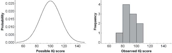
The examples presented in this paper use a set of Intelligence Quotient (IQ) measurements that were generated from a normal population with a mean of 100 and standard deviation of 15 (Figure 1, left panel). A small sample of 10 IQ scores from this population was randomly selected (Figure 1, right panel). A much smaller sample than is typical for behavioural research is used here to keep the examples mathematically simple.
Figure 1
Example of a population distribution (left panel) and the frequency plot of a small sample taken from that population (right panel). The sample contains 10 scores (see individual data in the text); they are grouped into bins of 10 points
Definition of Likelihood
The concept of Likelihood slowly emerged from the work of precursors such as Bernoulli and Gauss. It was first presented as a fully mastered concept in Fisher’s Statistical Methods for Research Workers (1925). Fisher’s ANOVA was created through the simplification of equations based on the Likelihood Method. Using Likelihood Ratios, Neyman and Pearson (1933) developed the concept of statistical power and demonstrated that t-tests and ANOVA tests are powerful test statistics when all of the assumptions are met.
Technically speaking, Likelihood is the probability that a population with a specified set of parameters was examined, given a sample of observations[1]. Differing from probabilities, which may be predictive (e.g., given a population A, what are the odds that a sample containing X and Y will occur?), Likelihood specifically refers to that which has already occurred (i.e., given that observations X and Y have occurred, how likely is it that this sample was taken from population A?). Thus, by definition, Likelihood can only be computed when a sample of observations from a population has already been collected.
Likelihood is mathematically noted with the uppercase script letter ℒ, and is generally written as follows:
where the x1, …, xn are a set of n observations, sometimes shortened to X and the vertical bar is read as «given the following observations». The population considered must have specific (and specified) characteristics. Using Likelihood, it is possible to calculate the likelihood of being in London, England, given that three successive days of rain have been observed from the vantage point of the laboratory window (highly likely). Later, it will be possible to compare this likelihood to the likelihood of being in Tamanrasset in the south of Algeria, given the same data (far less likely).
If a researcher is studying rainy days in a given city, the population is a description of how days are distributed between «rainy» and «non-rainy» (the binary measure in this situation). Thus, the term population is used to identify and describe quantifiable relevant characteristics – parameters – that describe the context in which the observations were sampled. While it is fairly simple in this example to calculate the proportion of days that are rainy vs. non-rainy based on an operational definition, the exact attributes of most populations are typically far more complex, and in many cases are entirely unknown. To quantify and describe unknown population parameters, hypotheses (models) are generated. Researchers may formulate several models for any definable construct. Thus, there is a need to determine which model, among many, best represents the data. Restated: Which of these hypothetical models has the best relative fit, or is the most likely to be a true representation of the population, given that this specific set of data were observed?
Another way to conceptualize Likelihood is to think of it as a probability measure bounded between zero and one. A value of zero indicates that a certain population parameter is extremely unlikely (to the point that it is impossible) and a value of one indicates that the specified parameter is absolutely likely (a certainty). Thus, Likelihood is the probability of the predefined population parameters being correct, given the observed characteristics of a situation.
Consider the case where there is only one observation. If the observation is collected from a known population, it is possible to compute the probability of the event. For example, if the characteristics of the present location are known (geographic location: London, England), and the objective is to determine tomorrow’s weather, the relevant characteristic is the probability of a rainy day given this location. Let us assume that the probability is 2/3 (or a 66% chance) that any day in London will be rainy. If, on the contrary, the objective is to determine one’s location based on an observation of rain, the probability appropriateness of being in London, given that is it raining at this moment, is 2/3 (providing that the above assumption is correct).
This can be summarized as:
Equation 3 uses statistical terminology, but is otherwise the same:
A population, in and of itself, is an abstraction. In the present context, it is only of interest to determine the probability of obtaining a given observation or datum in a specified population. The most prominent theoretical population is the normal distribution which is represented mathematically as 𝒩(μ,𝜎2) where the parameter μ is the mean, and 𝜎 is the standard deviation. The standardized version of the normal distribution is also known as the Gaussian distribution, where μ = 0 and 𝜎 = 1. A primary characteristic of a normally distributed population is that it is symmetrical about the mean: that is, observations smaller than the mean are equally as frequent as observations larger than the mean.
One difficulty with the normal distribution function is that it cannot be used to assign a probability to an extremely precise event. For example, with IQ scores, it is possible to know the probability of observing an IQ between 85 and 115, between 99 and 101, or even between 99.9 and 100.1, but the probability that it is precisely 100 is null (a score of 100.0000… is impossible) because possible IQ scores are continuous (a person’s score may fall anywhere on a continuum) rather than discrete (i.e., it is either raining now or not). When working with continuous data, the probability density is used to return the density of probabilities in a certain area describing a section of an underlying continuous scale. Here, we use the probability density function because we typically assign an integer to describe a participant’s IQ score, rather than determine his/her IQ to be precisely 120.005. For the normal distribution, the probability density function, noted conventionally with the letter f, is given by:
where e is the natural logarithm approximately equal to 2.71828. In the following sections, we use the term probability to refer to both probabilities and probability densities
As mentioned previously, in most applications, the actual value of the population parameter of interest is unknown. Therefore, Likelihood is computed using an assumption of hypothetical population parameters. When population normality is assumed, the Likelihood function is further simplified. For example, if it is assumed that all possible observations of the population parameter IQ are from a normal distribution that has a mean μ = 100 and standard deviation 𝜎 = 15, the probability of observing a given IQ having a value of x, under this model, can be computed by inserting the IQ value of interest, as shown in Equation 5. Note, again, that while IQ scores are typically reported as integers, the trait producing the IQ score is continuous, thus it requires that the probability density function be used.
Using the probability density function for a continuous variable, as shown in Equation 4, the probability of observing an IQ of 99, given the above model of the population, is .0265 or 2.65%. Conversely, if an IQ of 99 has already been observed, the probability (2.65%) is equal to the likelihood that the observation came from a population that was normally distributed with the mean μ = 100 and the standard deviation 𝜎 = 15. Equation 5 describes the relationship between the probability of observing a certain score, given a population, and the likelihood of a particular population given that a specific score has been observed.
Typically, a sample contains more than a single observation and for these the Likelihood is the joint probability of all of the individual observations. If the sample is comprised of independent observations, joint probability is found by calculating the product of the probabilities for each individual observation (Equation 6).
The probability values are numbers between 0 and 1. Multiplying several values smaller than 1 on a computer may yield a number that is indistinguishable from zero (an underflow error). For example, the likelihood of observing a sample of four IQs of 99 would be .02654 = .000000493 and for five observations it would decrease to .02655 = .000000013. Considering this, it is easy to understand how quickly these values become extremely small with sample sizes that are typical of behavioural research. Although the origins of using log values predate modern computing, calculating the log of likelihood – log(ℒ) – can be useful to avoid underflow and also because the log of a product is turned into a sum of logs (log(a × b) = log(a) + log(b). The sample log likelihood is then calculated by summing the logs of the individual likelihoods (Hélie, 2006). Using the log of likelihoods also frequently results in equations that are simpler. Note that log likelihoods are always negative values (but will change to positive values when calculating AIC and BIC as discussed in a latter section of this paper). See Example 1 in the Appendix for code in R to compute the log likelihood of a sample taken from a normally distributed population.
The log likelihood that the following 10 data (shown in Figure 1):
come from a normally distributed population with a mean of 100 and a standard deviation of 8, is -39.953, and this value is called the Log Likelihood Index (see Example 1 in the Appendix). For convenience, the log likelihoods are calculated in the examples. A log likelihood very close to zero indicates that the selected value for the parameter of interest (a mean of 100 in this example) is very likely. Conversely, a log likelihood index that is an extreme negative value would indicate that the assumed parameter is highly unlikely. The size of the calculated Likelihood Index is not only a function of how likely the sample is, but also a function of sample size. Thus, in isolation, it is impossible to say whether -39.953 is a “good” or “bad” result, but we may note that the actual mean of this sample is 92 and not 100, to give some meaning to the -39.953 for the purposes of this discussion. This will be elaborated upon in a subsequent section, where log likelihoods are used to compare the relative goodness-of-fit of differing models.
Using Maximum Likelihood to Estimate Parameters
In cases where the population is assumed to be of a certain distribution (e.g., normal distribution) but a given parameter is unknown, that parameter may be estimated by incrementally testing several possible values until the one that makes the assumed population most likely is found. This method of estimation is called the Maximum Likelihood Estimation (MLE) method. Using the sample X from the previous section, the parameter to be estimated is the population mean μ. The process of using the MLE method to compute differing values for μ until a “most likely” value for μ is found is given in Table 1 (with the value 𝜎 fixed at 8, arbitrarily).
Table 1
The results of using a Simplex algorithm to automate the search for the log likelihood values associated with the most likely population mean, given the sample data. The most likely value, of the values examined in this table, is the one whose log likelihood is closest to zero. (Here, that value closest to zero is associated with a mean of 92.)

See Example 5 for additional information.
Given these data, the best-fitting μ seems to be located close to 92. If a manual search were continued within the range 90 to 94, using smaller increments, 92.00 would be found after a few iterations. Instead of performing these computations manually, a maximization program, such as the Solver add-in in Excel, can be used to automate the search (Excel’s Solver uses the Simplex algorithm; Nelder & Mead, 1965). Alternately, Example 5a provides a short simulation in R that may also be used locate the most likely value for μ. The code given in Example 5b replicate the values in Table 1.
A way to visualize parameter estimation using MLE is to draw a plot of the log likelihood as a function of the hypothesized μ. Figure 2, left panel, shows an example in which 𝜎 is fixed at 8; in the right panel is an example where both μ and 𝜎 are varied. The shaded cross-section, where 𝜎 = 8, corresponds, and is equivalent to, the curve in Figure 2, left panel. In the right panel, the arrow indicates the “peak” of the dome, or the point at which the value being tested returns the highest (maximum) likelihood value.
Figure 2
One-way ANOVA output for data sets X and Y

Locating the maximum value that will satisfy a given argument can be summarized with the following notation:
in which μ represents the estimate of the parameter μ and the operator argmax represents any algorithm that can search for a maximum over all possible real values of μ.
Using Likelihood Ratios to Compare Models
Because many populations are so vast that the population characteristics of interest are not practical to collect as a whole, or are entirely unknown, researchers need a method to determine whether a hypothesized parameter is likely to represent the population of interest. In this scenario, what the researcher wants to know is “How likely is my presumed population parameter, (e.g., μ = 100), from this observed sample?” In less scientific language a researcher may ask: “Is my presumption about this population parameter likely to be accurate, given this sample that I have collected?” To answer this query mathematically, the researcher needs to determine how likely the parameter of interest is, given the set of collected data. Returning to scientific verbiage, the researcher’s hypotheses about the characteristics of a population are models that need to be evaluated. Frequently, several models are developed for a single population parameter. For example: “Is the population μ = 92 (equal to the mean of my sample)?” vs. “Is the population μ = 100, which is the generally accepted mean for IQ?” Thus, it is of value to be able to compare these models to determine which is the better fit, given the observations. One method of model comparison is to compute a Likelihood Ratio. In this context, the Likelihood Ratio is an index of the fit of one hypothetical model relative to another, given the observed sample.
Continuing with the observed IQ scores used in the previous examples, assume that the population mean is unknown. These two hypotheses may be generated from the aforementioned research questions: H1: The population is normally distributed with a mean of 92, and H2: The population is normally distributed with a mean of 100. Using Formula 4, the two likelihoods are computed as 643.7 × 10⁻¹⁸ for H1 and 6.95 × 10⁻¹⁸ for H2. For both hypotheses, let us assume that the parameter 𝜎 (the population’s standard deviation) is the same as the observed standard deviation of the sample, 8.41. With the sample likelihood for H1 in the numerator and the sample likelihood for H2 in the denominator, the resulting ratio is 92.6.
As mentioned earlier, log likelihoods simplify these computations, and yield equivalent conclusions. Here, the log likelihoods for H1 and H2 are -34.98 and -39.51 respectively. The Likelihood Ratio is obtained with: exp (log likelihood H1: – log likelihood H2:). For these log likelihood values, the ratio of log likelihoods can be obtained by entering: exp(-34.98 – (-39.51)) or: exp(4.53) = 92.7 directly into R or Excel. (Note that in Excel the exponent function must be preceded by “=”) Due to rounding errors, the last digit given here is an approximation.
The Likelihood Ratio is an indication of model fit. As calculated above, using either likelihoods or log likelihoods, the Likelihood Ratio calculated for model H1: μ = 92 vs. H2: μ = 100, is 92.7 to 1. Ratios of 20 to 1 can be likened to p value of 0.05; and can be interpreted to suggest that there is fair evidence in favour of the selected model. If likelihoods are used, this is the model whose fit is in the numerator; if log likelihoods are used to simplify computation, this is the first value entered into the subtractive equation (in the example, log likelihood H1). Ratios of 100 to 1 are similar to a p value of 0.01, and thus would represent even stronger evidence for the model (Glover & Dixon, 2004). Here, the ratio is nearly 100 to 1 in favour of H1. This result suggests that the model assuming μ = 92 is a better fit than the model μ = 100.
Conversely, a Likelihood Ratio that is close to one provides no evidence in favour of one model over another (i.e., a 1:1 ratio suggests that neither model is a better fit). When the Likelihood Ratio is greater than one, it favours the model whose likelihood is in the numerator (or is positioned first in the subtraction for log likelihoods); and when it is less than one, it favours the model whose likelihood is in the denominator (the model positioned second in the subtraction for log likelihoods). In this case, inverting the ratio (or switching the position of the log likelihood values) will yield the magnitude of support for the alternate model. For example, if the calculation above is changed to: exp (-39.51-(-34.98)) = .01. A Likelihood Ratio of .01 to 1 indicates no support for H2 as a better fit than H1 (which is correct, as the 92.7:1 ratio favoured H1 as the better fit).
Nested Models
As illustrated in the previous example, a researcher is able to determine that the fit of one model is superior to that of a competing model using the Likelihood Ratio. If one model is a nested version of the other, it is possible to determine if one model is a significantly better fit than another model. Calculated sample likelihoods for each model may be evaluated for statistical significance using a critical value gleaned from the𝜒2 distribution. This analysis can be conducted only in cases where models are nested and one has a free parameter while the competing model has this same parameter fixed, as described in the case below.
A researcher may need to determine whether the observations of IQ listed above are from a regular population – which in the case of IQ scores would be normal distribution with the parameter μ = 100. Here, the parameter μ is fixed a priori (i.e., given previous studies indicating that the population mean for IQ should be around 100). In this example, the alternative model is that the researcher believes μ = 100 is outdated and hypothesizes that the population’s mean is 92 instead, based upon an observed sample mean of 92. Here, μ is not fixed a priori because it is derived from the observations and, in statistical terms, μ is free to vary. Thus, the first model is a nested version of the second because both models are examining the same population parameter μ, and in one model μ is fixed, while in the alternate model μ varies from that fixed value. These models are defined as nested because they evaluate the same parameter(s). Models that differ in the number of parameters examined, or that explore differing parameters altogether are, therefore, not nested.
The method for comparing nested models is to calculate a Likelihood Ratio and then transform it into a test statistic, the Likelihood Ratio Test (LRT). Twice the natural log of the ratio resembles the distribution, with the degrees of freedom corresponding to the number of parameters that are free to vary in the nested model. As there is one parameter that may vary in this example, a critical value can be obtained from a table, with the degrees of freedom equal to one. In equations, there are two ways to compute LRT:
Returning to the IQ data given above, we compared the following two models:
The model Mfree contains a free parameter (the observed mean) and the model Mnested contains the fixed parameter μ = 100. The two models are identical except for the hypothesized value for the parameter μ. The observed sample mean is 92.0, and we have already computed the two likelihoods, -34.98 and -39.51, as well as the Likelihood Ratio, -92.7. Twice the base e log of the Likelihood Ratio (4.53) is 9.06. When this value is compared to 3.84, the critical value taken from a 𝜒2 (1) distribution at 𝛼 = 0.05, it is clear that 9.06 is larger. Therefore, it is possible to significantly reject Mnested in favour of Mfree, p < 0.05 (Chernoff, 1954). To obtain the p value of this significance test, obtain the probability that a 𝜒2 score with one degree of freedom exceeds 9.06, (shown in the last line of Example 2). For this example, p = 0.0026. Example 2 in the Appendix gives code to calculate the Likelihood Ratio using log likelihoods and performs a test of significance for the hypothesized mean vs. a fixed population mean in a single sample.
Model comparisons that use twice the log of the likelihood ratio are based on asymptotic arguments. Thus, the 𝜒2 table provides only approximate critical values when the sample sizes are small (n < 30). More accurate decision thresholds are obtained when the sample size is increased toward infinity, as 𝜒2 critical values become more precise.
Note also that the square root of 9.06 is 3.01. This quantity is found when computing the t statistic for a Student’s t-test with the null hypothesis: H0: μ = 100, 𝛼 = 0.05. This relationship is explained further in the section Maximum Likelihood vs. Other Estimation Approaches. Likewise, taking the square root of the critical value, 3.84, yields 1.96, which is the critical value of a t-test when the sample size is infinite (and also the critical value of a z-test).
Adjustments using AIC and BIC
In the previous section using nested models, model complexity was controlled for because the models being compared were identical except for one free parameter. While the likelihoods of nested models are directly comparable, the likelihoods of non-nested models cannot be directly compared, and in many cases it is of interest to compare models with differing parameters. When the two models to be compared are not nested, there is no single correct method to compare their likelihoods, as the comparison of likelihoods depends on model complexity.
Model complexity is the ability of a model to fit any data. Complexity is strongly influenced by the number of free parameters; therefore, counting the free parameters is a heuristic measure of model complexity. Thus, as the number of free parameters increases, the model complexity increases as well, and the goodness-of-fit also improves. As a result, some models, particularly those with several parameters, are capable of fitting almost any sample. As the purpose of developing models is usually to explain a particular facet of or phenomenon in a given population, a model that seems to fit all data sets because it is overly complex is considered to be over-fitted. As such, an over-fitted model may include so many parameters that it is of little use to explain the outcome score that is of interest.
To prevent over-fitting, models with a higher number of free parameters should be penalized before the likelihoods are compared (Hélie, 2006). Several methods of imposing this penalty have been proposed: AIC, AIC-corrected, AIC3, the constrained AIC criterion, BIC, DIC, and WICVC to name a few (Akaike, 1974; Bozdogan, 1987; Hélie, 2006; Wu, Chen, & Yan, 2013). Of these, we will briefly discuss AIC, AIC- corrected, and BIC and how these relate to computations of Likelihood.
The Akaike Information Criterion (AIC) of a model is based on its Likelihood and is computed with:
where k is the number of the model’s free parameters, and ℒ (as above) is the likelihood, or measure of fit for a model with a given set of parameters to a sample (Akaike, 1974; Hélie, 2006). Note that log likelihoods are typically negative numbers and the multiplier -2 in the AIC calculation changes the sign to positive. Therefore, the model that yields an AIC value closer to zero is the model with the better relative fit. The penalty term 2k moves the fit away from zero in proportion to the number of free parameters in the model. To simplify, the primary concept of the AIC is that it imposes a “fit penalty” that is proportional to the number of free parameters in a given model so that there is less “over-fitting” when the number of parameters examined in a model is increased.
Using the IQ dataset above, the AIC value for the models μ = 92 and μ = 100 may be calculated as: AIC = -2 × (-34.98) + 2 × 1 = 71.96 and AIC = -2 × (-39.51) + 2 × 1 = 81.02 respectively. To determine the relative Likelihood of these models, in Equation 9, ℒ is replaced with AIC, thus, exp ((AICmax — AICmin) /2) = 92.7 where AICmax is the largest AIC value calculated for the models being examined (ℒ = -39.51, AICmax = 81.02) and AICmin is the calculated AIC for the instance of the model that is being compared (ℒ = -34.98, AICmin = 71.96). In the present case, because both models are of the same complexity (one free parameter) the penalties cancel out and the same result as above, exp(4.53) = 92.75, is obtained.
The AIC index is only valid with large sample sizes, as the AIC is biased for small samples (i.e., the AIC value calculated in these cases is overestimated); thus, there is a need to reduce it, or add an additional penalty for small samples. Therefore, for smaller sizes, the AIC-corrected (AICc) can be used. Hurvich and Tsai (1989) developed the AICc as a bias-corrected version of the AIC for cases where sample sizes are small (n < 100) or where the number of free parameters is large (k > 5). The AICc formula is as follows:
where n is number of observations, k is the number of free parameters, and AIC is the AIC value as calculated above. In short, the AICc contains an additional penalty term that increases as a function of the number of parameters in the model. The purpose of the additional penalty is to reduce the AIC overestimation bias that occurs for small sample sizes. It can be seen that as sample sizes increase, the second penalty term vanishes and, thus, AIC and AICc converge to the same value. It may also be noted that when the models being considered have the same number of parameters (k), comparing models using AIC and AICc yields identical results. Therefore, in such a case, AICc affords no additional benefit over AIC, yet there is no adverse consequence of applying the AICc as it will yield an equivalent model evaluation.
The Bayesian Information Criterion (BIC), also known as the Schwarz criterion (Schwarz, 1978), has also been developed to compensate for model complexity by adding a penalty term based on the number of parameters in a given model, therefore preventing over-fitting. The BIC assumes that model errors are independent, normally distributed, and homoscedastic (i.e., the error of prediction does not depend on the scores to be fitted, thus are relatively equal within a given group). Similar to the AICc, the BIC was developed to suit smaller samples; however the BIC imposes a stricter (larger) penalty. BIC is computed as follows:
The BIC is fairly analogous to the AIC except that the penalty term is based on both the number of free parameters and the sample size. The logic behind this correction is that the model becomes less flexible as a function of sample size. That is, it is progressively more constrained by the data as the sample size increases. When two models are compared using this method, the model with the lower calculated BIC is interpreted to be the better fit, or the more likely correct, for the given models (Schwarz, 1978).
Burnham and Anderson (2004) recommend using the AIC to the exclusion of BIC, based upon the idea of multimodel interference, the philosophy of information theory, and the principle of parsimony. To briefly summarize their recommendation, the AIC is preferred over the BIC because the model selected by the AIC will be more parsimonious (be more general/simpler) and the model returned by BIC will be more complex (include more free parameters).
Nested Models vs. Model Adjustments
The adjustments (AIC, AICc or BIC) allow any given model to be compared to any other model. However, these adjustments are only approximately adjusting for complexity. More precise adjustments exist (see Grünwald, 2000; Myung, 2000), but they are often impossible to compute. Conversely, nested model comparisons are based on solid mathematical foundations. Therefore, the statistical significance of a nested model over a general model cannot be disputed. It is worth noting that although two models may seem unrelated, it is sometimes possible to develop a generalized model which includes the two competing models as special cases/sub-models. See Heathcote, Brown, and Mewhort (2000), and Smith and Minda (2002) who used this approach to study learning curves and categorization processes, respectively. Developing a generalized model is advantageous because it can be used to assess the importance of one sub-model relative to another in terms of the model’s ability to explain the data.
Finally, a caution must be noted here. While the AIC, BIC and Likelihood Ratio calculations can inform the researcher which of two models is the most likely, or the best fit, these indices cannot provide any information about the overall quality of a model taken in isolation. It is always possible that all of the models being evaluated are poor models. Thus, these formulae can only be applied to determine which model is the best fit among those being evaluated.
Advantages and Limitations of the Likelihood Approach
Estimating parameters using Maximum Likelihood Estimation (MLE), as described previously, is not a guarantee for success (Cousineau, Brown, & Heathcote, 2004). However, statisticians have established the following properties of the method (see Rose & Smith, 2001).
Advantages of MLE: Consistency, Normality, and Efficiency
As sample sizes increase, the estimate tends towards the true population parameter. Thus, for a more accurate estimate, a larger sample is preferable to a smaller. As sample sizes increase, the error of estimation is normally distributed. As a consequence, easier-to-apply test statistics (e.g., t tests, ANOVA) can be used on a set of estimates. Also, as sample sizes increase, no other method can been found to estimate the parameter(s) of a model more efficiently than MLE. For small samples, alternatives to MLE have been proposed, but for very large samples, the benefit of applying a more time-intensive alternative is marginal. These three properties are considerable advantages; because of this, MLE underlies most (if not all) current statistical tests. It must be noted that MLE does, however, have two important limitations: non-regular distributions and biased estimation.
Limitations
Non-regular distributions are models where a parameter value is constrained by a single observed value. One example is the Weibull model, which is commonly used to describe psychophysics data (e.g., in Nachmias, 1981): the position parameter of this distribution has to be smaller than the smallest observation. Conversely, the normal distribution is a regular distribution where μ and 𝛼 are not constrained by any one observation. Many distributions are non-regular. For non-regular distributions, there may be no maximum likelihood, or there may be several maximum likelihoods – which invalidates the concept of maximizing likelihood. It is not always easy to identify non-regular distributions. (See Kiefer, 2005, for a complete list of criteria that must be satisfied before a model can be declared regular). As MLE is inapplicable for the analysis of non-regular populations, there are alternative methods that can be applied. A few of these are discussed briefly in the section entitled Alternatives to Likelihood.
The second important limitation of MLE is that the estimates that are obtained using this method are often biased. That is, they contain a systematic error of estimation. The amount of bias depends on sample sizes and tends to zero as sample size is increased toward infinity (the consistency property, above). However, for small samples, estimate bias can be substantial. A prominent example of this is the normal population’s standard deviation. The usual method to estimate 𝛼 is to divide the sum of the squared deviations by (n - 1). However, when solving MLE analytically, the solution requires the sum of squared deviations to be divided by n. Once it was realized that the results of MLE were biased in this case, a solution to produce an unbiased estimate was found: divide the sum of squared deviations by (n - 1) instead of n (see Cousineau, 2010, or Hays, 1973, for a demonstration).
To illustrate MLE estimation bias in further detail, note that in Figure 1, left panel, the maximum is located under the point 92 (on the μ axis) and 7.97 (on the 𝛼 axis). This second number is biased downward. The bias is corrected by multiplying 7.97 by ![]() (replacing the division by n with a division by (n - 1) returning 8.40. This method to correct for bias when estimating the standard deviation, however, is only applicable to normally distributed models. This correction for bias using (n - 1) is also used to compute sum of squares in the ANOVA or correlations whenever the assumption of normality is invoked.
(replacing the division by n with a division by (n - 1) returning 8.40. This method to correct for bias when estimating the standard deviation, however, is only applicable to normally distributed models. This correction for bias using (n - 1) is also used to compute sum of squares in the ANOVA or correlations whenever the assumption of normality is invoked.
The disadvantage resulting from estimate biases may outweigh the advantages outlined above. Thus, when evaluating estimators, finding and correcting the amount of bias (if any) in the MLE approach is one of the first tasks. Unfortunately, biases are present for most parameters in the vast majority of models (the parameter μ of the normal distribution is a rare exception). Additionally, expressing the specific amount of bias is often impossible, thus correcting for bias may be also impossible with particular models (see Cousineau, 2009, for a successful example with the Weibull model).
Maximum Likelihood vs. Other Estimation Approaches
Least Squares Modeling and the Assumption of Normality
The assumption of normality implies that the data are normally distributed: i.e., the data fit the normal distribution, whose probability function was given in Equation 1. The normal probability density function is based on an exponentiation. Therefore, when computing the log likelihood of a single datum, both operators cancel out; thus the following simpler formula is obtained:
It can be noted from the first term in Equation 13 that this formula is based on the sum of squared deviations between the observations and the parameter μ. Expressed verbally, every time a sum of squares is computed, this computation is a log likelihood function assuming normality. This concept did not escape R. A. Fisher’s notice: he presented the ANOVA technique using the sum of squares, as the sum of squares is much easier to compute manually than Likelihood (Fisher, 1925). However, the two approaches are mathematically equivalent, and return the same F statistic.
As an example, consider two samples:
The most general model would assume that two distinct populations were sampled to obtain X and Y; and that these two populations may have distinct means. The best estimates for each population mean are the observed means of each sample: that is, 92.0 and 100.0, respectively. A restricted model would assume that both populations are identical and, consequently, have an equal mean. The best estimate of the population mean for the restricted model is the grand mean, or the average of all the observations (96.0), irrespective of whether they come from X or from Y. Following Fisher, the exact value of the standard deviation for each group is not relevant, therefore, the pooled standard deviation is used (spooled = 11.78).
The log likelihood for the X and Y samples with respect to Mfree is -76.70 whereas the log likelihoods with respect to Mnested is -77.85. The Likelihood Ratio: exp(-76.70 - (-77.85)) is 3.16. This indicates approximately three times more support for the free model as compared to the nested model. LRT is twice the log of the ratio between these two values: that is, 2.31. However, this quantity is not larger than the 𝜒2(1) critical value 3.841; therefore, the free model’s fit is better, but not significantly better, than the nested model. Example 3 in the Appendix provides R code to perform these calculations.
The same data, analyzed using an ANOVA yields the results shown in Table 2.
Table 2
One-way ANOVA output for data sets X and Y

Note that the F ratio is identical to the model comparison index that was calculated above. The exact critical value for F (1, 18) is 4.414, which is slightly larger than the approximate 𝜒2(1) critical value found earlier. For larger sample sizes, the F critical values converge toward the 𝜒2 critical values. For example, F (1, 36) = 4.113, F (1, 180) = 3.894, F (1, 1800) = 3.846 and F (1, 18,000) = 3.842. The log likelihood and sum of squares are equivalent whenever the normal distribution is assumed. This is true for regression (simple or multiple), for mediation and moderation, and for structural equation modeling as well. This is why these analyses are often grouped under the generic term: Least Squares Modeling – all of these were created from model comparisons based on Likelihood.
While it is not a necessity that data be normally distributed in order to perform statistical analyses, the normal distribution is the only distribution that enables the computation of log likelihoods using the sum of squared deviations (a much simpler formula). The relative ease of applying these formulae is likely the reason that these analyses became so prevalent in the early days of statistics. Now, however, with the advent of fast computing, replacing the normality assumption with any other assumption regarding the family of distribution is a trivial manipulation. Example 4 in the Appendix provides code demonstrating how to replace the normality assumption with the Cauchy distribution (a symmetrical distribution with thicker tails, which allows for the presence of extreme values).
Bayesian Inference
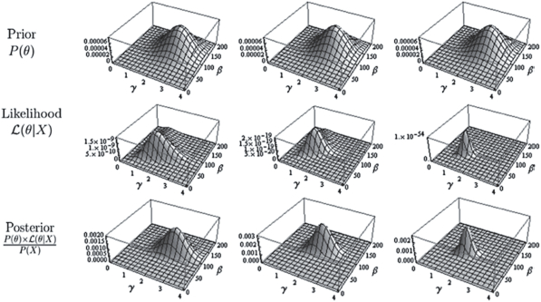
Bayesian Inference is an extension of the likelihood method with the addition of one supplement: priors, or prior probabilities. In order to conduct a Bayesian analysis, priors must first be specified. A prior is an a priori expression giving the probability that a certain parameter can take a specific value (e.g., the probability that it will be a rainy day in London). After a sample is collected, the priors are revised using the likelihood function. This “fine tuning” of the priors is called updating, and returns a posterior. In an ideal world, the new posteriors would become priors before a new sample is collected, leading to a second round of updating, etc. Figure 3 illustrates one round for three different samples. In this figure, the three priors are the same, but the sample sizes are tiny, very small, and small. As a result, the maximum likelihood becomes more peaked, resulting in more concentrated posteriors. Both the priors and the posteriors are expressed in the form of a distribution that indicates a degree of belief in certain values of the parameters composing the model. In the special case where the priors assume that the parameters to be estimated can take any value with the same probability (this is labeled «no priors») and in that case only, both the most probable Bayesian estimate and maximum likelihood estimate return the same value.
Figure 3
(top row) Examples of a prior, expressed with a distribution over the parameters (here 𝛾 and 𝛽); (middle row) likelihood functions for a very small, small or moderate sample sizes; (bottom row) posterior, found by multiplying the above two lines. Taken from Cousineau and Hélie, (2013)
Bayesian Inference can be challenging to apply to behavioural data for two reasons. First, it is difficult to express prior beliefs regarding certain parameters, particularly when those parameters relate to subjective human constructs. For example, how does one formulate a degree of belief with regard to a parameter affecting well-being? Additionally, in empirical practice, posteriors from one study rarely become the new priors of another investigation, as each researcher prefers to state their own prior probabilities. Second, the likelihood must be weighted by a “normalization” term (as indicated in Note 1) which weighs the current sample with respect to all possible samples. Unfortunately, it is often impossible to quantify the normalization terms as this involves solving multiple integrals. Numerical approximations are possible using, for example, techniques based on the Monte Carlo Markov Chain (Hadfield, 2012). These, however, can be time consuming to compute and may yield divergent results. A compromise is to ignore the normalization term. This solution may be used if only the location of the maximum is required: i.e., to get a posterior in the form of a single estimate) instead of the distribution of an estimate. Approaches such as these have been proposed: Maximum likelihood estimation with A Priori (MAP; Birnbaum, 1969), and Prior-informed Maximum Likelihood Estimation (piMLE; Cousineau & Hélie, 2013).
Alternatives to Likelihood
As mentioned above, piMLE can be used to expand likelihood estimation with priors. Other alternatives to MLE are: Maximum Product of Spacing (MPS), Maximum Product of Quantiles (MPQ), and weighted Maximum Likelihood Estimation (wMLE). The MPS approach, developed by Cheng and Amin (1983), was specifically created for non- regular models. In this approach, it is not the probability of the individual datum that is used to compute probabilities, but the spacing between two successive data points. This method is reliable in every situation and can be used with success when MLE is not applicable. MPS also tends to return less biased estimates. The MPQ approach, created by Brown and Heathcote (2003; also see Heathcote, Brown, & Cousineau, 2004) bases its estimation on quantiles of data. Because individual data are replaced by quantiles of the data, this method is less sensitive to outliers. It is therefore a robust equivalent of MLE (Daszykowksi, Kaczmarek, Vander Heyden, & Walczak, 2007). MPQ, however, is sensitive to non-regular distributions. Lastly, wMLE, created by Cousineau (2009) is not truly an approach based on MLE, although it does return pseudo-MLE estimators. These estimators are identical to MLE except for the introduction of weights for the purpose of canceling biases. The wMLE method is applicable irrespective of the type of distribution (regular or non- regular), returns unbiased estimators, and has been tested for various models by Nagatsuka, Kamakura, and Balakrishnan (2013) and Ng, Luo, and Duan (2011).
Conclusion
In the social sciences, researchers are often confronted with the challenge of applying statistical tests that require population parameters that are unknown (e.g., the population mean). Due to the impracticality or impossibility of collecting data from the entire population, the researcher can posit that the population mean is equal to a specified value. It can then be determined how likely it is that this value is accurate, given an observed sample. One method that can be applied to evaluate a hypothetical population mean is to calculate the likelihood of the sample using the likelihood function. Another practical application of the likelihood function is that it may be used to conduct model comparisons to determine the relative likelihood of two or more nested hypotheses to determine which of these is the best fit, given the observed data.
The relationship between Likelihood and Student’s t test and Fisher’s ANOVA are discussed here, and mini-proofs are given in the examples. Likelihood can also be used to estimate regression slopes. Multiple regression uses MLE and, as a result, the formulae used known as the Least Squares Methods were developed. In Hierarchical Linear Modeling (HLM; Woltman, Feldstein, MacKay, & Rocchi, 2012) and Structural Equation Modeling (SEM; Weston & Gore, 2006), the use of Least Squares Modeling formulae is not possible; thus, all of these analyses are explicitly based on MLE.
Many modern test statistics assume data normality and variance homogeneity (homoscedasticity). Real-world behavioural data, however, is often non-normal and the within-group variances are never exactly homogeneous. Collected samples are often rich with outliers, or clusters of data that pose normality problems, and then the researcher is burdened with deciding whether it is ethical to discard valid outliers in order to perform statistical tests. These inherently challenging characteristics of psychological data can create ethical grey areas or require complicated data transformations; thus, certain data can be difficult to analyze statistically. Likelihoods can be used to attenuate these challenges.
Likelihood is also very useful in model construction and in the process of simplifying overly complex models. Once the best-fitting parameters of a given model are identified, they can be set to zero one by one; and if the resulting model is equivalent (in terms of fit) to the best-fitting model, it implies that the said parameter is not necessary to capture the trends seen in the data. The model can then be simplified accordingly; this approach is automated in stepwise regression (Cohen & Cohen, 1975). When researchers are not required to perform complex data transformations or make difficult decisions regarding whether to include or discard valid outliers, they are able to more effectively analyze real-world data where the underlying populations are not best-represented by the normal distribution. As a result, higher quality, better fitting models can be generated.
Parties annexes
Appendix
Appendix. Examples in R
The present apendix provides five examples of computation done in the R statistical environment (version 3.0.2, 64-bit) to compute Likelihood for model comparisons and parameter estimation. Please note that while on some computer systems, code can be copied directly from a pdf document to R, not all systems recognize the carriage returns (“enters” at the end of each line). If errors are encountered in copying and running any of the following examples, this can be solved by copying the text first into a text editor program, such as Notepad++ for the PC, or Xcode or Tincta for the Mac, and confirming that the lines of code have not been blended together (by going to the end of each line and adding an extra “enter”).
1. Computing the log likelihood from a sample, assuming a normal population:
# define the data into a vector.
data <- c(79, 84, 85, 87, 87, 97, 99, 99, 101, 102)# compute the log likelihood;
# dnorm represents the normal probability density function,
# mean and sd represents the parameters 𝜇 and 𝜎 respectivelylogL <- sum( log( sapply(data, dnorm, mean = 100, sd = 8 )))
# a line of code to display the results
cat("log likelihood for this set of data = ", logL)
2. Testing a hypothesized mean for a single group, assuming a normal population:
In this example, the models are identical except that in one case (Model 1), the mean is the sample mean, 92, whereas in Model 2, the mean is the default mean for a population of IQ, 100.
# define the data into a vector.
data <- c(79, 84, 85, 87, 87, 97, 99, 99, 101, 102)# compare two models with parameter sigma set to the observed standard deviation
logL1 <- sum( log( sapply(data, dnorm, mean = 92,. sd = sd (data) )) )
logL2 <- sum( log( sapply(data, dnorm, mean = 100, sd = sd (data) )) )# the likelihood ratio
r <- exp(logL1 - logL2)# the model comparison; in this case, the square root is same as t
F <- 2 * (logL1 - logL2) # same as LRT
t <- sqrt(F)# get the p value for the found F
pval<-pchisq(F, 1, lower.tail = FALSE)# a line of code to display the results
cat("log likelihood for this set of data at ",mean(data), " = ", logL1,"\nlog likelihood for this set of data at mean = 100 = ", logL2,"\nLikelihood Ratio= ",r,"np-value = ",pval,"\nANOVA F= ",F,"\nStudent’s t= ",t)
3. Using likelihood to determine if two groups are from the same population:
This example examines whether two samples come from a single population or two distinct populations. In either case, the population(s) are assumed to be normally distributed (normality assumption) and if there are two populations, it is assumed that they share the same parameter (homogeneity of variances assumption). To test for this, two models are generated (one being a nested version of the other) and compared using likelihood ratio. This is the exact logic that underlies the ANOVA test.
# define two data sets into vectors.
IQ1 <- c(79, 84, 85, 87, 87, 97, 99, 99, 101, 102)
IQ2 <- c(71, 84, 91, 99, 100, 104, 110, 112, 114, 115)# getting the pooled standard deviation as per regular approach
sp <- sqrt( ((length(IQ1)-1) * var(IQ1) + (length(IQ2)-1)
*var (IQ2)) / (length(IQ1) + length(IQ2)-2))# compute the general model with one parameter per group, using observed means
logL1 <- sum( log( sapply(IQ1, dnorm, mean = mean(IQ1), sd = sp ) ) ) +
sum( log( sapply(IQ2, dnorm, mean = mean(IQ2), sd = sp )) )# compute the nested model, with a single mean for all the data
logL2 <- sum( log( sapply(IQ1, dnorm, mean= mean
(append(IQ1,IQ2)), sd = sp))) +
sum( log( sapply(IQ2, dnorm, mean=mean(append(IQ1,IQ2)), sd = sp)))# the likelihood ratio
r <- exp(logL1 - logL2)# the model comparison; in this case, the square root is same as t
F <- 2 * (logL1 - logL2) # same as LRT
t <- sqrt(F)# a line of code to display the results
cat("log likelihood for IQ1= ", logL1,"\nlog likelihood for
IQ2= ",logL2,"\nLikelihood Ratio= ",r,"\nANOVA F=
",F,"\nStudent’s t= ",t)
4. Running a test of mean on a single group, not assuming a normal distribution
The normal distribution is a mesokurtic distribution, which means that extreme values are very rare in this theoretical population. However, in psychology, extreme values (outliers) are not that rare. This contradicts the normality assumption. Classical approaches to the problem of outliers are (a) to remove the extreme values, or (b) to transform the data to increase their conformity to a normal population. An alternative solution presented here is to assume a population distribution that better fits the data. To accommodate the presence of the extreme values, a distribution with longer tails is needed. One such distribution is the Cauchy distribution (Forbes, Evans, Hastings, & Peacock, 2010). It has parameters μ and 𝛽. The parameter μ is the mean of the distribution and the second parameter, 𝛽, is a scale parameter roughly equal to two-thirds of the standard deviation. It can be estimated by taking half the interquartile range of the data (IQR / 2).
In the example below, IQ is examined. The objective is to determine if the group mean IQ is as usual for the general population, 100. The sample contains one extreme value (154), but after verification, the number is valid and the researcher is reluctant to eliminate this datum. Running a regular t-test in R with: t.test(IQs, mu = 100), the result is not significant (t(9) = 1.61, p = .142) suggesting a lack of evidence: This group seems to have nothing unusual even though the sample mean, 109.6, is unusually high. The extreme value, however, has inflated the sample’s standard deviation, and in turn has increased the standard error. The inflation of these values may mask a significant difference that otherwise would be found. The following solves the issue without discarding the outlier.
In the general model fitted below, the mean is free to vary and is set to the observed mean; and in the nested model, the mean is set to 100. Note that everything is identical to the second example above, except that the normality assumption (computed using the function dnorm) is replaced by a Cauchy assumption (computed using the function dcauchy), which accommodates outliers because the tails of the distribution are longer (in technical terms, the Cauchy distribution is leptokurtic). Thus, in this case, the Cauchy distribution is a more correct approximation of a population containing outliers than the normal distribution in which these values are rare.
# define the IQ data into a vector.
IQs <- c(79, 101, 101, 102, 106, 110, 113, 114, 116, 154)# compare two models with parameter beta set to the interquartile range
logL1 <- sum( log( sapply(IQs, dcauchy, location = mean(IQs), scale = IQR(IQs)/2 )) )
logL2 <- sum( log( sapply(IQs, dcauchy, location = 100, scale = IQR(IQs)/2 )) )# the likelihood ratio
r <- exp(log L1 - logL2)# the model comparison result
F <- 2 * (logL1 - logL2)
The F observed is 5.069, larger than the 𝜒2(1) critical value (3.841). Hence, there is evidence after all suggesting that the sample does not come from a population that has a mean IQ of 100. Note that this last conclusion is the correct one as this sample was computer-generated from a population whose mean was 105.
5. Finding best-fitting parameters using R:
This set of examples shows a few ways that best-fitting parameters can be searched/estimated. It implements what was called “argmax” in Equation 7. It is a maximization/optimization procedure that can be applied to obtain the maximum value that satisfies a given argument.
5a. A Simplex Algorithm in R (the Nelder & Mead method)
IQ <- c(79, 84, 85, 87, 87, 97, 99, 99, 101, 102)
# We define the log likelihood as a function;
# theta is a vector containing the two unknown parameters 𝜇 and
𝜎 logl <- function(theta, data) {
sum( log( sapply(data, dnorm, mean = theta[1], sd = theta[2] )))
}constrOptim(
# here we provide some initial values to the parameters more or less randomly
theta = c(100,10),# this is the function to maximize, with no gradient provided
f = logl,
grad = Null,# constraints: just one is needed (sigma must be larger than zero)
ui = matrix(c(0,1),1),
ci = c(0,0),# use simplex and run maximization (default is minimization)method="Nelder-Mead",
control=list(fnscale=-1),# what follows is additional parameters for the function logl data = IQ)
5b. An R Simulation to Produce Table 1 (MLE to estimate the population mean)
This example creates a sequence of possible μ where the likelihood must be evaluated. Currently, the possible μ are between 80 and 100, by Step of 2 (80, 82, 84, …, 100); you can reduce the range and the step sizes to narrow the search on Line 2 of the code.
data <- c(79, 84, 85, 87, 87, 97, 99, 99, 101, 102)
LIST_OF_MUS <- seq( 80, 100, by = 2)
# The researcher may change the bounds and precision in the line of code above# initialize empty output collector vectors
MU_COLLECTOR<-c()
LOGL_COLLECTOR<-c()#*****************ITERATION START****************************
for (POSSIBLE_MU in LIST_OF_MUS) {
# compute the loglikelihood;
logL <- sum( log( sapply(data, dnorm, mean = POSSIBLE_MU, sd = 8 )))# collect the results
MU_COLLECTOR <- append(MU_COLLECTOR, POSSIBLE_MU)
LOGL_COLLECTOR <- append(LOGL_COLLECTOR, logL)
}#***************ITERATION FINISHED************************
# display results
OUTPUT.COLLECTED<-data.frame(MU_COLLECTOR, LOGL_COLLECTOR)
OUTPUT.COLLECTED
Note
-
[1]
To be precise, Likelihood is proportional to the probability of a certain population given a sample. A constant is required but this constant does not depend on the observations, and therefore, can be ignored in all the applications of Likelihood.
References
- Akaike, H. (1974). A new look at the statistical model identification. IEEE Transactions on Automatic Control, 19(6), 716–723. doi: 10.1109/TAC.1974.1100705
- Birnbaum, A. (1969). Statistical theory for logistic mental test models with a prior distribution of ability. Journal of Mathematical Psychology, 6, 258-276. doi: 10. 1016/ 0022-2496(69)90005-4
- Bozdogan, H. (1987). Model selection and Akaike’s information criterion (AIC): The general theory and its analytical extensions. Psychometrika, 52(3), 345-370. doi: 10.1007/BF02294361
- Brown, S., & Heathcote, A. (2003). QMLE: Fast, robust and efficient estimation of distribution functions based on quantiles. Behavior Research Methods, Instruments, & Computers, 35, 485-492. doi: 10.3758/BF03195527
- Burnham, K., & Anderson, D. R. (2004). Multimodel interference, understanding AIC and BIC in model selection. Sociological Methods & Research, 33(2), 261–304. doi: 10.1177/0049124104268644
- Cheng, R. C. H., & Amin, N. A. K. (1983). Estimating parameters in continuous univariate distributions with a shifted origin. Journal of the Royal Statistical Society B, 45, 394–403. doi: 10.2307/2345411
- Chernoff, H. (1954). On the distribution of the likelihood ratio. The Annals of Mathematical Statistics, 25(3). 573-578. doi: 10.1214/aoms/1177728725
- Cohen, J., & Cohen, P. (1975). Applied Multiple Regression/correlation analysis for the behavioral sciences. Hillsdale, NJ: Lawrence Erlbaum Associates.
- Cousineau, D. (2009). Nearly unbiased estimates of the three-parameter Weibull distribution with greater efficiency than the iterative likelihood method. British Journal of Mathematical and Statistical Psychology, 62, 167–191. doi: 10.1348/000711007X270843
- Cousineau, D. (2010). Panorama des statistiques pour psychologues. Bruxelles, Belgique: Les éditions de Boeck Université.
- Cousineau, D., Brown, S., & Heathcote, A. (2004). Fitting distributions using maximum likelihood: Methods and packages. Behavior Research Methods, Instruments, & Computers, 36, 742–756. doi: 10.3758/BF03206555
- Cousineau, D., & Hélie, S. (2013). Improving maximum likelihood estimation using prior probabilities: Application to the 3-parameter Weibull distribution. Tutorials in Quantitative Methods for Psychology, 9, 61–71.
- Daszykowksi, M., Kaczmarek, K., Vander Heyden, Y., & Walczak, B. (2007). Robust statistics in concept analysis - A review: Basic concepts. Chemometrics and Intelligent Laboratory Systems, 85, 203–219. doi: 10.1016/j.chemolab.2006.06.016
- Fisher, R. A. (1925). Statistical Methods for Research Workers. Edinburgh, Scotland: Oliver and Boyd.
- Forbes, C., Evans, M., Hastings, N., & Peacock, B. (2010). Statistical Distributions. New York, NY: Wiley.
- Glover, S., & Dixon, P. (2004). Likelihood ratios: A simple and flexible statistic for emprical psychologists. Psychonomic Bulletin & Review, 11, 791–806. doi: 10.3758/BF03196706
- Grünwald, P. (2000). Model Selection based on minimum description length. Journal of Mathematical Psychology, 44, 133–152. doi: 10.1006/jmps.1999.1280
- Hadfield, J. D. (2012). MasterBayes: Maximum Likelihood and Markov chain Monte Carlo methods for pedigree reconstruction, analysis and simulation. Retrieved from: http://cran.r-project.org/web/packages/.
- Hays, W. L. (1973). Statistics for the social sciences. New York, NY: Holt, Rinehart and Winston, Inc.
- Heathcote, A., Brown, S., & Cousineau, D. (2004). QMPE: Estimating lognormal, Wald and Weibull RT distributions with a parameter dependent lower bound. Behavior Research Methods, Instruments, & Computers, 36, 277–290. doi: 10.3758/BF03195574
- Heathcote, A., Brown, S., & Mewhort, D. J. K. (2000). The power law repealed: The case for an exponential law of practice. Psychonomic Bulletin & Review, 7, 185–207. doi: 10.3758/BF03212979
- Hélie, S. (2006). An introduction to model selections: Tools and algorithms. Tutorials in Quantitative Methods for Psychology, 2, 1–10.
- Hurvich, C. M., & Tsai, C. L. (1989). Regression and time series model selection in small samples. Biometrika, 76(2), 297–307. doi: 10.2307/2336663
- Kiefer, N. M. (2005). Maximum likelihood estimation (MLE), Retrieved from: http://instruct1.cit.cornell.edu/courses/econ620/reviewm5.pdf
- Myung, I. J. (2000). The importance of complexity in model selection. Journal of Mathematical Psychology, 44, 190–204. doi: 10.1006/jmps.1999.1283
- Nachmias, J. (1981). On the psychometric function for contrast detection. Vision Research, 21, 215–223. doi: 10.1016/0042-6989(81)90115-2
- Nagatsuka, H., Kamakura, T., & Balakrishnan, N. (2013). A consistent method of estimation for the three-parameter Weibull distribution. Computational Statistics and Data Analysis, 58, 210–226. doi: 10.1016/j.csda.2012.09.005
- Nelder, J. A., & Mead, R. (1965). A simplex method for function minimization. The Computer Journal, 7, 308–313. doi: 10.1080/00401706.1975.10489269
- Neyman, J., & Pearson, E. S. (1933). On the problem of the most efficient tests of statistical hypotheses. Philisophical Transactions of the Royal Society of London. Series A, Containing Papers of a Mathematical of Physical Character, 231, 289–337. doi: 10.1098/rsta.1933.0009
- Ng, H. K. T., Luo, L., & Duan, F. (2011). Parameter estimation of three-parameter Weibull distribution based on progressively type-II censored samples. Journal of Statistical Computation and Simulation, 10, 1-18. doi: 10.1080/00949655.2011. 591797
- Rose, C., & Smith, M. D. (2001). Mathematical Statistics with Mathematica. New York, NY: Springer-Verlag.
- Schwarz, G. (1978). Estimating the dimension of a model. The Annals of Statistics, 6(2), 461–464. doi: 10.1214/aos/1176344136
- Smith, J. D., & Minda, J. P. (2002). Distinguishing prototype-based and exemplar-based processes in dot-pattern category learning. Journal of Experimental Psychology: Learning, Memory and Cognition, 28, 800–811. doi: 10.1037/0278-7393.28.4.800
- Weston, R., & Gore, P. A. Jr. (2006). A brief guide to structural equation modeling, The Counseiling Psychologist, 34, 719–751. doi: 10.1177/0011000006286345
- Woltman, H., Feldstain, A., MacKay, J. C., & Rocchi, M. (2012) An introduction to hierarchical linear modeling, Tutorials in Quantitative Methods for Psychology, 8, 52–69.
- Wu, T.-J., Chen, P., & Yan, Y. (2013). The weighted average information criterion for multivariate regression model selection. Signal Processing, 93, 49-55. doi: 10.1016/S0167-7152(98)00003-0
Liste des figures
Figure 1
Example of a population distribution (left panel) and the frequency plot of a small sample taken from that population (right panel). The sample contains 10 scores (see individual data in the text); they are grouped into bins of 10 points
Figure 2
One-way ANOVA output for data sets X and Y
Figure 3
(top row) Examples of a prior, expressed with a distribution over the parameters (here 𝛾 and 𝛽); (middle row) likelihood functions for a very small, small or moderate sample sizes; (bottom row) posterior, found by multiplying the above two lines. Taken from Cousineau and Hélie, (2013)
Liste des tableaux
Table 1
The results of using a Simplex algorithm to automate the search for the log likelihood values associated with the most likely population mean, given the sample data. The most likely value, of the values examined in this table, is the one whose log likelihood is closest to zero. (Here, that value closest to zero is associated with a mean of 92.)
See Example 5 for additional information.
Table 2
One-way ANOVA output for data sets X and Y