Résumés
Abstract
The underground waters in the Mamundiyar basin, India, present real chemical quality problems. Their fluoride content always exceeds the recommended levels. The Inverse Distance Weighted (IDW) method has been used for spatial interpolation of various key chemical parameters. Artificial Neural Network (ANN) modeling was applied to understand the correlation and sensitivity of all chemical parameters with respect to fluorides. The correlation of all the considered parameters is found to be poor where the highest correlation observed was only 0.37. This result showed that four of the parameters, namely pH, chlorides, sulphates and calcium, were found to have greater capacity of influencing fluorides than the other eight parameters. Chlorides were found to be the parameter that was the most sensitive and most correlated to fluorides.
Keywords:
- Fluoride,
- Groundwater,
- Artificial Neural network,
- Inverse Distance Weighted,
- Mamundiyar basin
Résumé
Les eaux souterraines du bassin de Mamundiyar (Inde) présentent des problèmes avérés de qualité chimique. Leur teneur en fluorures dépasse toujours les valeurs recommandées. La méthode de la Pondération Inverse à la Distance (PID) a été utilisée pour interpoler spatialement différents paramètres chimiques. Une modélisation par réseaux de neurones artificiels a été ensuite appliquée pour comprendre les corrélations et niveaux de sensibilité de tous les paramètres chimiques par rapport aux fluorures. Il y a un faible degré de corrélation entre les paramètres, le plus grand coefficient étant seulement de 0,37. Les quatre paramètres qui influencent le plus les fluorures sont le pH, les chlorures, les sulfates et le calcium. La teneur en chlorures est le paramètre le plus corrélé aux fluorures.
Mots-clés :
- Fluorures,
- Eaux souterraines,
- Réseaux de neurones artificiels,
- Pondération Inverse à la Distance,
- Bassin de Mamundiyar
Corps de l’article
1. Introduction
The hydrology and geochemistry of waters have been discussed in the classic works of STUMM and MORGAN (1981), HEM (1991), DREVER (1988), DOMENICO and SCHWARTZ (1990), DAR et al., (2009, 2012, 2010a, b, 2011), but the occurrence of fluoride in groundwater has drawn worldwide attention due to its considerable impact on human physiology. About 80% of the diseases in the world are due to poor quality of drinking water (WHO, 1984). Large groups of people in the following countries suffer from fluorosis due to intake of F- rich groundwater: Argentina, U.S.A, Morocco, Algeria, Libya, Egypt, Jordan, Turkey, Iran, Iraq, Kenya, Korea, Tanzania, S. Africa, China, Australia, New Zealand, Japan, Thailand, Canada, Saudi Arabia, Sri lanka, Syria and India (APAMBIRE et al.; 1997, BINBIN et al., 2005; DISSANAYAKE, 1991; GRIMALDO et al, 1995; MEENAKSHI and MAHESHVERI, 2006; SHOMAR et al., 2004; ZHANG et al., 2003).
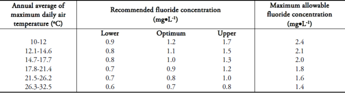
The problem of excessive fluoride in groundwater in India was first reported in 1937 in the state of Andhra Pradesh. In India, approximately 62 million people including 6 million children suffer from fluorosis because of consumption of water with high fluoride concentrations. Seventeen states in India have been identified as endemic for fluorosis and Tamil Nadu is one of them. Though fluoride enters the body through food, water, industrial exposure, drugs, cosmetics, etc., drinking water is the major contributor (75-90% of daily intake). According to the World Health Organization (WHO, 1971) permissible limit for fluoride in drinking water is 1.0 mg•L-1, whereas the United States Public Health Services has set a range of allowable concentrations for fluoride in drinking water for a region depending on its climatic conditions because the amount of water consumed and consequently the amount of fluoride ingested being influenced primarily by the air temperature (USPHS, 1987). The maximum allowable fluoride concentrations as established by USPHS are shown in Table 1. Accordingly, the maximum allowable concentration for fluoride in drinking water in Indian conditions comes to 1.4 mg•L-1 while, as per Indian standards, it is 1.5 mg•L-1.
Table 1
Range of maximum allowable fluoride concentrations as specified by the USPHS.
Gamme des concentrations maximales en fluorures permises selon l’USPHS.
Being the most electronegative element, Fluorine has the tendency to acquire a negative charge and form fluoride ion (F-) in solution. F- ions have the same charge and nearly the same radius as that of hydroxide ions and may replace each other in mineral structure. F- ions thus form mineral complexes with number of cations and some common species of low solubility contain F- ions (HEM, 1991). Besides the environmental concern of fluoride in natural waters, the deduction of the ultimate source of fluoride and establishing the mode of dissolution together with transport in natural waters and natural sinks of the fluoride ion are issues which need to be addressed. Keeping aside the anthropogenic sources, such as burning of coal, extraction of aluminum, steel industries and using phosphate-based fertilizers which are potential sources of fluorine, natural sources (such as leaching of rocks and enriched soils) involve speculation beyond a certain extent. Fluorite (CaF2) is the only principal mineral of fluoride, mostly present as accessory minerals in granitic, and occasionally in alkaline rocks (e.g. syenite and nepheline syenites). Apatite, amphiboles and micas, which are ubiquitous in igneous and metamorphic rocks, contain fair amounts of fluorine in their structure. Sedimentary horizons also have apatite as an accessory mineral and fluorite also often occurs as cement in some sandstones. Therefore, all these are natural contributors to fluoride in fluids interacting with them, such as groundwater, thermal waters and surface waters. However, while the geochemistry of fluorite solubility in natural water is known (NORDSTORM and JENNY, 1997), there is not much work on the quantitative evaluation of fluoride in groundwater, especially in mineral-fluid equilibrium. The occurrence of high concentrations of fluoride in groundwater (1.5 mg•L-1) in the Nayagarh district of Orissa, India, and its relation with the fluoride-rich hot spring water (more than 10 mg•L-1) have been studied by KUNDU et al., (2001). APAMBIRE et al. (1997) studied the geochemistry of fluoriferrous groundwater in the upper region of Ghana, India and ascribed the fluoride contamination qualitatively to the presence of coarse-grained hornblende granites and syenite in the area. These authors suggested dissolution of fluorite and anion exchange with micaceous minerals and their clay alteration products as the cause of fluoride enrichment. Hydrochemical processes controlling the occurrence of fluoride in groundwater include solution precipitation reaction, adsorption-desorption processes, and dispersion of chemical formation complex and abundance of fluorine in source rocks studied by LLOYD (1985). A better understanding of fluoride geochemistry in the aquatic environment under specific geographic and geologic conditions is very necessary for evaluating the contamination process. This may help in the long run to propose new and more efficient remedial measures to combat the threat.
The main objectives are: (1) to study the spatial variation of F- in the groundwater of Mamundiyar basin, and (2) to understand the controls on the spatial distribution of F- and other ions in groundwater.
2. Geography and geology of the study area
The Mamundiyar River Basin is the area chosen for the present study. It extends over approximately 720 km2 and lies between 10o 25' and 10o 40' N latitudes and 78o 10' and 78o 30' E longitudes in the central part of Tamilnadu, India (Figure 1). It falls within three districts viz., Tirucherapalli, Dindugul and Pudukottai. Mamundiyar River originates at an altitude of 315 m above Irungadu group of hills and joins Ariyavur River near Maravanur about 25 km southwest of Tiruchirapalli. The western, northwestern and southwestern parts are characterized by the presence of residual hills. The basin is generally hot and dry except during winter season. The mean maximum monthly temperature varies from 32.77oC in May to 25.5oC in December. While as mean minimum monthly temperature ranges from 27.2oC in May to 18.87oC in December. The area receives an average annual rainfall of about 678.24 mm. The surface runoff goes to stream as instant flow. Rainfall is the direct recharge source and the irrigation return flow is the indirect source of groundwater in the Mamundiyar River Basin. The study area depends mainly on the northeast monsoon rains which are brought by the troughs of low pressure established in the Bay of Bengal. It forms a part of the Survey of India (SOI) topographic sheets of 58J/2, J/3, J/6, J/7, and J/10 on a scale of 1:50,000.
Figure 1
Location of the study area.
Localisation de la zone d’étude.

Several digital image processing techniques, including standard color composites, intensity-hue-saturation (IHS) transformation and decorrelation stretch (DS) were applied to map rock types. The statistical technique adopted by SHEFFIELD (1985) was employed to select the most effective three-band color composite image. The band combination 1, 4 and 5 is the best triplet and was used to create color composites with Landsat TM bands 5, 4 and 1 in red, green and blue, respectively. IHS transformation and DS were also applied to the selected band combination in order to enhance the difference between rock types. Better contrast was obtained due to color enhancement and this facilitated visual discrimination of various rock types. Eleven lithologic units were mapped and could be distinguished by distinct colors in the processed images. These are: Ultramafics, Hornblende biotite gneiss, Basic rocks, Charnockite, Pyroxene granulite, Pink magmatite, Quartzite, Pegmatite vein, Quartz vein, Granite, and Calc granulite and limestone.
3. Methodology
3.1 Inverse Distance Weighted (IDW) method
For estimation of groundwater quality of unsampled locations, spatial interpolation was required with a satisfying level of accuracy. There are many spatial Interpolation algorithms for spatial (2-D or 3-D) data sets. DEUTSCH and JOURNEL (1998) discuss in detail kriging, GOODMAN and O’ROURKE (1997) splines, ZURFLUEH (1967) trend surfaces, and HARBAUGH and PRESTON (1968) Fourier series. LAM (1983) gives a review and comparison of spatial interpolation methods. There are two categories of Interpolation techniques, deterministic and geostatistical. Deterministic Interpolation technique creates surfaces based on the measured points or mathematical formulae. Methods such as IDW are based on extent of the similarity of cells while geostatistical Interpolation such as kriging is based on statistics and used for more advance prediction surface modeling that also includes some measure of accuracy of the prediction. Kriging is similar to IDW in the sense that it uses a weighting that assigns more influence to the nearer data points to interpolate values at unknown locations. However, instead of using the IDW approach, kriging uses variograms. As a measure of spatial variability, a variogram replaces the Euclidean distance by a structural distance that is specific to the attribute and the field under study, (DEUSTSH and JOURNEL, 1998). For spatial correlation, a perfect semivariogram is required for which parameters can be determined. The geochemical data in the study area are non-stationary because many of the closely located points have values drastically different from each other. Because of this, the IDW method has been used for interpretation of data instead of kriging in order to generate maps of continuous maps of geochemical parameters.
IDW interpolation determines cell values using a linearly weighted combination of a set of sample points. The weight is a function of inverse distance. The farther an input point is from the output cell location, the less importance it has in the calculation of output value. Because the IDW is the weighted distance average, the average cannot be greater than the highest or lower than the lowest input. Therefore it can not create ridges or valleys if these extremes have not already been sampled.
Also, because of averaging, the output surface will not pass through the sample points. The best results obtained from the IDW are obtained when sampling is well distributed to represent the local variation that needs to be simulated. In IDW the measured values (known values) closer to prediction location will have more influence on the predicted value (unknown value) than those farther away. More specifically, IDW assumes that each measured point has a local influence that diminishes with increase in distance. Thus, points near in the neighborhoods are given high weights, whereas, points at far distance are given small weights (LIXIN, 2004). The general formula of IDW interpolation is the following (JOHNSTON et al., 2001):
where w(x,y) is the predicted value at location (x,y), N is the number of nearest known points surrounding (x,y), li are the weights assigned to each known point value wi at location (xi,yi), di are the Euclidean distances between each (xi,yi) and (x,y), and P is the exponent, which influences the weighting of wi on w. In the present study, a p value of 2 and a search radius of 5000 m have been used for interpolation.
3.2 Artificial Neural Network (ANN) modeling
Artificial Neural Network (ANN) modeling was used to understand the Correlation and sensitivity of all parameters with respect to Fluoride. A total of five (5) models were developed in order to understand the correlation and sensitivity of the water quality parameters with respect to fluoride. The five models (Table 2) developed are:
Development of the First model with ‘Highest Sensitive to Fluorine’ Parameters (HSY): pH, Chloride (Cl), Calcium (Ca) and Sulphate (SO4);
Development of the Second model with ‘Highest Correlated with Fluorine’ Parameters (HCR): Chloride (Cl), Bicarbonate (HCO3), Nitrate (NO3) and Sodium (Na);
Development of the Third model with the Highest Correlated and Sensitive Parameter with respect to Fluorine (SSHCRSY): Chloride (Cl);
Development of the Fourth model with those parameters which was not considered in the above three models (NHSY): Electrical Conductivity (EC), Total Dissolved Solids (TDS), Magnesium (Mg), Sodium (Na), Potassium (K) and Phosphate (PO4);
Development of the Fifth model with all the parameters (ALL): Chloride (Cl), Bicarbonate (HCO3), Nitrate (NO3), Sodium (Na), Electrical Conductivity (EC), Total Dissolved Solids (TDS), Magnesium (Mg), Sodium (Na), Potassium (K) and Phosphate (PO4).
Table 2
Performance validation criteria for the neuro-genetic models developed.
Critères de performance en matière de validation pour les modèles neuronaux développés.

3.2.1 Development of the neuro-genetic models
ANNs are flexible mathematical structures that are capable of identifying complex nonlinear relationships between input and output data sets. ANNs offer a relatively quick and flexible means of modeling and as a result, the application of ANN modeling was widely reported in various hydrological literatures. These networks are “neural” in the sense that they may have been inspired by neuroscience but not necessarily because they are faithful models of biologic neural or cognitive phenomena.
3.2.1.1 Mathematical representation of Artificial Neural Network
The ANN model of a physical system can be considered with n input neurons (x1,x2...xn), h hidden neurons (z1,z2..zn) and m output neurons (y1,y2...yn). Let tj be the bias for neuron zj and fk for neuron yk. Let wij be the weight of the connection from neuron xi to zj and beta is the weight of the connection zj to yk. The function that ANN calculates is:
in which:
where gA and fA are the activation functions.
The development of an artificial neural network, as prescribed by ASCE (2000), follows the following basic rules:
Information must be processed at many single elements called nodes;
Signals are passed between nodes through connection links and each link has an associated weight that represents its connection strength;
Each of the nodes applies a non-linear transformation called as activation function to its net input to determine its output signal.
The number of neurons contained in the input and output layers are determined by the number of input and output variables of a given system. The size or number of neurons of a hidden layer is an important consideration when solving problems using multilayer feed-forward networks. If there are fewer neurons within a hidden layer, there may not be enough opportunity for the neural network to capture the intricate relationships between indicator parameters and the computed output parameters. Too many hidden layer neurons not only require a large computational time for accurate training, but may also result in overtraining. A neural network is said to be “over-trained” when the network focuses on the characteristics of individual data points rather than just capturing the general patterns present in the entire training set.
3.2.1.2 Methodology for development of neuro-genetic models
Figure 2 showed a basic diagram of neural network topology. The development of neuro-genetic models can be divided into four phases which are described below:
Figure 2
Schematic diagram of an artificial neural network.
Schéma de principe d’un réseau de neurones artificiels.

Phase 1: Data preprocessing
The first step in the development of neuro-genetic models is to preprocess the data so that the models can include it for training. Dataset is required to be scaled and normalized before using it to train the model. If the dataset is not normalized, then much processing power and time will be wasted by the model to convert the dataset into binary. The dataset is also required to be scaled so that data anomalies and overrides can be avoided.
Phase 2: Selection of network topology
Neural networks can be of different types, like feed forward, radial basis function, time lag delay, etc. The type of the network is selected with respect to the knowledge of input and output parameters and their relationship. Once the type of network is selected, selection of network topology is the next concern. Trial and error method is generally used for this purpose but many studies now prefer the application of genetic algorithm (AHMED and SARMA, 2005). Genetic algorithms are search algorithms based on the mechanics of natural genetic and natural selection.
Genetic algorithm is a robust method of searching the optimum solution to complex problems like the selection of an optimal network topology where it is difficult or impossible to test for optimality. The basics of GA have already been discussed by many authors like AHMED and SARMA (2005), WANG (1991), WARDLAW (1999). Hence the details of the basic procedures of GA are not given in the present paper.
Phase 3: Training phase
To encapsulate the desired input output relationship, weights are adjusted and applied to the network until the desired error is achieved. This is called “training the network”.
Phase 4: Testing phase
After training is completed, some portion of the available historical dataset is fed to the trained network and known output is estimated out of them. The estimated values are compared with the target output to compute the MSE. If the value of MSE is less than 1%, the network is said to be sufficiently trained and ready for estimation. The dataset is also used for cross-validation to prevent over-training during the training phase. (MAJUMDER, 2009). Model characteristics of the neuro-genetic models developed for the present study is shown in Table 3. All the models are trained with Levenberg-Marquardt and the information related to the architecture and training and testing MSE are given in Table 3.
Table 3
Model characteristics of the neuro-genetic models developed.
Caractéristiques des modèles neuronaux développés.

4. Results
The samples were collected in 1-liter polyethylene bottles from the 50 sites of the study area. Measurements of electrical conductivity and pH were carried out in situ using a portable conductivity meter (Cond 330i/ SET, WTW, Germany) and a portable pH meter (pH 315i/ SET, WTW, Germany). Samples were collected in clean polyethylene bottles and dispatched for analysis to the laboratory (Soil Testing Laboratory, Trichy, Tamil Nadu) in an ice-filled box. In the laboratory, samples were refrigerated at 4°C and the analysis was carried out within 48 h of collection.
The values obtained for various physico-chemical parameters after carrying out the analysis of the ground water samples are presented in Table 4.
Table 4
Statistical analysis of various parameters.
Analyse statistique des différents paramètres.

The abundance of major ions in groundwater was found in the following order:
Ca > HCO3 > Cl > Mg > SO4 > Na > F > K > NO3 > PO4
The pH values varied from 6.96 – 7.65 (7.24 ± 0.16) indicating slightly acidic-alkaline nature.
The sodium and bicarbonate values varied from 20 to 96 and 80 to 189 mg•L-1 respectively. The fluoride concentration varied from 0.61 – 6.59 (3.33 ± 1.02) with highest fluoride level at SE part (6.59 mg•L-1). The concentration of fluoride found in the ground water samples (except sample number 44) was higher compared to the Indian Drinking Water Standard of maximum permissible limit of 1 mg•L-1 and the maximum tolerance limit (1.5 mg•L-1) recommended by WHO (2004) and the Bureau of Indian Standrads (BIS, 2003). The major source of fluoride is the fluorite mineral which may be found in granite, gneiss and pegmatite. The process of weathering of rock releases fluoride in soil and ground water. The alkaline water can mobilize fluoride from fluorite with precipitation of calcium carbonate because the solubility of CaF2 increases with an increase in NaHCO3 rather than with other salts (HANDA 1975; SAXENA and AHMED 2001). In ground water, the natural concentration of fluoride depends on the geological, chemical and physical characteristics of the aquifer, the porosity and acidity of the soil and rocks, the temperature, the action of other chemical elements, and the depth of wells. The aqueous ionic concentrations of ground water may influence the fluoride solubility behavior in the presence of excessive sodium bicarbonates and the dissociation activity of fluoride will be high (TIRUMALESH et al., 2007). In acidic form, fluoride is absorbed in clay, and in alkaline form, it is desorbed. Hence, alkaline pH is more favorable for fluoride dissolution activity and can be represented as:
In order to identify possible combinations, ratio values of different variables were studied, which are presented in Table 5. The ratio of HCO3/Cl was found in the range of 0.68 – 2.4 (1.11 ± 0.32). The average ratio value of 1.11 indicates dominance of carbonate ions, whereas values less than one indicate that chloride ion is prevalent in the region. The Na/Cl ratio was observed in the range of 0.12 - 0.43 (0.27 ± 0.09). The decrease in ratio indicates modification of sodium carbonate water by dissolution or mixing with sodium chloride, whereas increase in chloride may be due to local recharge. The ratio value of Na/Ca was observed in the range of 0.13 - 0.51 (0.26 ± 0.09). The increase in ratio value may be due to lowering calcium activity whereby high sodium activates the dissolution of fluoride bearing minerals at higher pH in groundwater system (SHAJI et al., 2007). The HCO3/Ca ratio observed in the range of 0.52 - 1.93 (1.04 ± 0.28) (values in meq), which indicate favorable chemical condition during fluoride dissolution process (SAXENA and AHMAD, 2003).
Table 5
Ratio and correlation values of different water quality variables.
Rapport et coefficients de corrélation des différents paramètres de qualité des eaux.

The geochemical evolution of groundwater can be understood by plotting the concentrations of major cations and anions in the PIPER (1994) trilinear diagram (Figure 3). On the basis of chemical analysis, groundwater is divided into six facies. The plot shows that the groundwater samples fall in the field of CaCl, CaHCO3 respectively, according to their order of their dominance.
Figure 3
Piper plot of the sample set.
Diagramme de Piper de l’ensemble des échantillons.

4.1 Correlation and sensitivity of various parameters w.r.t fluoride
In the present study, there are 12 quality parameters that have been measured along with fluorides. The objective was to identify the relationship between them and fluorides. In this regard, total five models were prepared where in one model all the 12 parameters are included to predict F sensitivity. In the second model, the top four most sensitive or influential parameters are included as input, the third model was prepared with the four most correlated parameters. The fourth model was developed with the most correlated and sensitive parameter as input. The last model was developed with the help of the last eight less sensitive parameters.
Table 6 shows the performance validation achieved for all five models where it can be seen that HSY model comes as the best model among all the five models considered. The model developed without the sensitive or correlated parameters comes last. This shows that the top four most sensitive parameters had considerable influence on the model output. Even the top four most correlated parameters have lesser influence on the output. Again only the top most sensitive parameter alone is not influencing the characteristics of the output variable as it is evident from the model performance where only 27.9% correlation, 2.30% error and 6.40% standard deviation were observed for the latter model. The correlation of all the considered parameters is found to be poor where the highest correlation was observed was only 0.370. This result showed that even if the relationship is poor, four of the parameters, namely pH, Cl, SO4 and Ca, were found to have greater capacity of influencing fluorine than the other eight parameters. Chloride is found to be the most sensitive and most correlated to fluoride.
Table 6
Sensitivity and correlation of the considered water quality parameters with fluoride.
Sensibilité et coefficients de corrélation des paramètres de qualité d’eau considérés avec les fluorures.

Although the correlation of the three most correlated parameters get increased and was found to be equal to -0.92, -0.59, -0.38 and -0.15 respectively for pH, Cl, SO4 and Ca with respect to the predicted Fluoride from the existing correlation values of -0.07, -0.29, -0.05 and -0.02.
4.2 Correlation of F- with other geochemical parameters
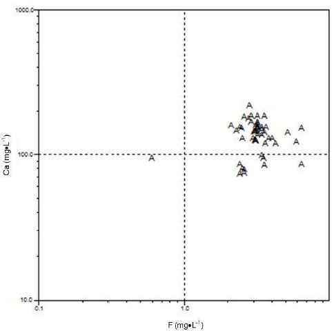
Scatter plots between F and other geochemical parameters (Cl, Mg, K, HCO3 and Ca) are shown in Figures 4-8.
Figure 4
Scatter plot of fluorides versus chlorides.
Fluorures en fonction des chlorures.
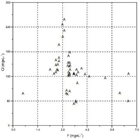
Figure 5
Scatter plot of fluorides versus magnesium.
Fluorures en fonction du magnésium.

Figure 6
Scatter plot of fluorides versus potassium.
Fluorures en fonction du potassium.

Figure 7
Scatter plot of fluorides versus bicarbonate.
Fluorures en fonction des bicarbonates.

Figure 8
Scatter plot of fluoride versus calcium.
Fluorures en fonction du calcium.
4.3 Spatial distribution of geochemical parameters
The spatial distribution of F- is shown in Figure 9. Using the IDW method, the spatial distribution of some important geochemical parameters is presented in Figures 10 to 14. It is envisaged that high weathering along the lineament might have resulted in increased dissolution of minerals in groundwater. The spatial distribution of F- indicating high level of F- in groundwater primarily occurs in southeastern and southwestern parts of study area.
Figure 9
Spatial distribution of fluorides.
Distribution spatiale des fluorures.

Figure 10
IDW-based spatial distributions: fluoride.
Distributions spatiales obtenues selon la méthode de pondération inverse à la distance: fluorures.
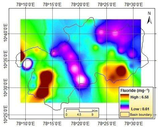
Figure 11
IDW-based spatial distributions: total dissolved solids.
Distributions spatiales obtenues selon la méthode de pondération inverse à la distance: solides totaux dissous.

Figure 12
IDW-based spatial distributions: bicarbonate.
Distributions spatiales obtenues selon la méthode de pondération inverse à la distance : bicarbonates.

Figure 13
IDW-based spatial distributions: calcium.
Distributions spatiales obtenues selon la méthode de pondération inverse à la distance: calcium.

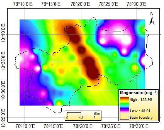
Figure 14
IDW-based spatial distributions: magnesium.
Distributions spatiales obtenues selon la méthode de pondération inverse à la distance: magnésium.
5. Conclusions
In the present study, the IDW method has been used for interpretation of data in order to generate maps of continuous maps of geochemical parameters. Almost all the parameters fall within the permissible limit except fluoride.
ANN modeling was done to understand the correlation and sensitivity of all parameters with respect to Fluoride. The correlation of all the considered parameters is found to be poor where the highest correlation observed was only 0.370. Even if the relationship was found to be poor, but four of the parameters, namely pH, Cl, SO4 and Ca, were found to have greater capacity of influencing fluoride than the other eight parameters. Chloride is found to be the most sensitive and most correlated to fluoride.
Parties annexes
Ackwnoledments
This paper is part of the primary author’s PhD research work. We thank reviewers for their constructive review of the manuscript and we are very much grateful to the Editor for editorial revision.
References
- AHMED J.A. and A.K. SARMA (2005). Genetic algorithm for optimal operating policy of a multipurpose reservoir. J. Water Resour. Manage., 19, 145–161.
- APAMBIRE W.B., D.R. BOYLE and F.A. MICHEL (1997). Geochemistry, genesis and health implication of fluoriferous groundwater in the upper regions, Ghana. Environ. Geol., 33, 13-24.
- ASCE Task Committee on Application of Artificial Neural Networks in Hydrology (2000). Artificial Neural Networks in Hydrology. I: Preliminary Concepts. J. Hydrol. Eng., 5, 115-123.
- BINBIN W., Z. BAOSHAN, W. HONGYANG, P. YAKUN and T. YUEHNA (2005). Dental carries in fluorine exposure areas in China. Environ. Geochem. Health, 27, 343-347.
- BIS (Bureau of Indian Standards) (2003). Drinking water specification IS: 10500, New Delhi, India.
- BURN D.H. and J.S. YULIANTI (2001). Waste-load allocation using genetic algorithms. J. Water Resour. Plan. Manage., ASCE, 127, 121-129.
- DAR I.A, M.A. DAR and K. SANKAR (2009). Nitrate contamination in groundwater of Sopore town and its environs, Kashmir, India. Arabian J. Geosci., 3, 267-272.
- DAR I.A, K. SANKAR and M.A. DAR (2010a). Investigation of groundwater quality in hardrock terrain using Geoinformation System. Environ. Monitor. Assess., 176, 575-595.
- DAR I.A, K. SANKAR and M.A. DAR (2010b). Spatial assessment of groundwater quality in Mamundiyar basin, Tamil Nadu, India. Environ. Monitor. Assess., 178, 437-447.
- DAR M.A, K. SANKAR and I.A. DAR (2011). Fluoride contamination - A major challenge. Environ. Monitor. Assess., 173, 955-968.
- DAR I.A, K. SANKAR, S. TANZEEM SHAFI and M.A. DAR (2012). Hydrochemistry of groundwater of Thiruporur block, Tamil Nadu (India). Arabian J. Geosci., 5, 259-262.
- DISSANAYAKE C.B. (1991). The fluoride problem in the groundwater of Srilanka - Environment management and health. Int. J. Environ. Stud., 38, 137-156.
- DEUTSCH C.V. and A.G. JOURNEL (1998). GSLIB: Geostatistical Software Library and user’s guide (2nd ed.). Oxford University Press, New York, NY.
- DOMENICO P.A. and F.W. SCHWARTZ (1990). Physical and chemical hydrogeology.Wiley (Éditeur), New York, NY, USA, pp. 410-420.
- DREVER J.I. (1988). The geochemistry of natural waters (2nd ed.), Prentice-Hall, New York, NY, USA, 437 p.
- GOODMAN J.E., and J. O’ROURKE (Eds.) (1997). Handbook of discrete and computational geometry. Boca Raton, CRC Press, New York, NY, USA, 1539 p.
- GRIMALDO M.B., V.H. RAMIREZ, A.L. PONCE, M. ROSAS and F. DIAZ BARRIGA (1995). Endemic fluorosis in San-Luis, Potosi, Mexico. Identification of risk-factors associated with human exposures to Fluoride. Environ. Res., 68, 25-30.
- HANDA B.K. (1975). Geochemistry and genesis of fluoride containing groundwater in India. Groundwater, 13, 278-281.
- HARBAUGH J.W. and F.W. PRESTON (1968). Fourier analysis in geology. Englewood Cliffs, Prentice-Hall, New York, NY, USA, pp. 218-238.
- HEM J.D. (1991). Study and interpretation of the chemical characteristics of natural water. Book 2254, 3rd ed., Scientific Publishers, Jodhpur, India, 263 p.
- JOHNSTON K., J.M.V. HOEF, K. KRIVORUCHKO and N. LUCAS (2001). Using ArcGIS geostatistical analyst. ESRI Press, Redlands, CA, USA, 48 p.
- KUNDU N., M.K. PANIGRAHI, S. TRIPATHY, S. MUNSHI, M. POWELL and B.R. HART (2001). Geochemical appraisal of fluoride contamination of groundwater in the Nayagarh district, Orissa, India. Environ. Geol., 41, 451-460.
- LAM N.S. (1983). Spatial interpolation methods: a review. Amer. Cartogr., 10, 129-149.
- LIXIN L. and P. REVESZ (2004). Interpolation methods for spatio-temporal geographic data. Comput. Environ. Urban Sys., 28, 201-227.
- LLOYD J.W. and J.A. HEATHCOTE (1985). Natural inorganic hydrochemistry in relation to groundwater. Clarendon Press, Oxford, UK, 296 p.
- MEENAKSHI M. and C. MAHESHVERI (2006). Fluoride in drinking water and its removal. J. Hazard. Mater., 137, 456-463.
- MAJUMDER M., R.N. BARMAN, B. JANA, P.K. ROY and A. MAZUMDAR (2009). Application of Neuro-Genetic Algorithm to determine reservoir response in different hydrologic adversaries. J. Soil Water Res., 4, 17-27.
- NORDSTORM D.K. and E.A. JENNY (1997). Fluorite solubility equilibria in selected geothermal waters. Geochem. Cosmochem. Acta, 41, 175-188.
- PIPER A. (1994). A graphic procedure in the geochemical interpretation of water analyses. Transac. Amer. Geophysical Union, 25, 83-90.
- SAXENA V.K. and S. AHMED (2003). Inferring the chemical parameters for the dissolution of fluoride in groundwater. Environ. Geol., 43,731-736.
- SHAJI E., B.J. VIJU and D.S. THAMBI (2007). High fluoride in groundwater of Palghat District, Kerala. Curr. Sci., 92, 240-246.
- SHEFFIELD C. (1985). Selecting band combinations from multispectral data. Photogram. Eng. Remot. Sens., 51, 681-687.
- SHOMAR B., G. MULLE, A. YAHYA, S. ASKAR and R. SANSUR (2004). Fluoride in groundwater soil and infused-black tea and the occurrence of dental fluorosis among the children of Gaza strip. J. Water Health, 2, 23-35.
- STUMM W. and J. MORGAN (1981). Aquatic chemistry (2nd ed.), Wiley, New York, NY, 1022 p.
- TIRUMALESH K., K. SHIVANNA and A.A JALIHAL (2007). Isotope hydrochemical approach to understand fluoride release into groundwaters of Ilkal area, Bagalkot District, Karnataka, India. Hydrogeol. J., 15, 589-598.
- USPHS (United States Public Health Services) (1987). Drinking water standards, Washington, DC, USA.
- WANG Q.J. (1991). The genetic algorithm and its application to calibrating conceptual rainfall-runoff models. Water Resour. Res., 27, 2467-2471.
- WARDLAW R. and M. SHARIF (1999). Evaluation of genetic algorithms for optimal reservoir system operation. J. Water Resour. Plan. Manage., 125, 25-33.
- WHO (1971). International standards for drinking water. Geneva, Switzerland, 1, 53-73.
- WHO (1984). Guidelines for drinking water quality. Geneva, Switzerland.
- WHO (2004). Guidelines for drinking water quality. 3rd ed., Geneva, Switzerland.
- ZHANG B., M. HONG, Y. ZHAO, X. LIN, X. ZHANG and J. DONG (2003). Distribution and risk assessment of fluoride in drinking water in the western plain region of Jilin province, China. Environ. Geochem. Health, 25, 421-31.
- ZURFLUEH E.G. (1967). Applications of two-dimensional linear wavelength filtering. Geophysics, 32, 1015-1035.
Liste des figures
Figure 1
Location of the study area.
Localisation de la zone d’étude.
Figure 2
Schematic diagram of an artificial neural network.
Schéma de principe d’un réseau de neurones artificiels.
Figure 3
Piper plot of the sample set.
Diagramme de Piper de l’ensemble des échantillons.
Figure 4
Scatter plot of fluorides versus chlorides.
Fluorures en fonction des chlorures.
Figure 5
Scatter plot of fluorides versus magnesium.
Fluorures en fonction du magnésium.
Figure 6
Scatter plot of fluorides versus potassium.
Fluorures en fonction du potassium.
Figure 7
Scatter plot of fluorides versus bicarbonate.
Fluorures en fonction des bicarbonates.
Figure 8
Scatter plot of fluoride versus calcium.
Fluorures en fonction du calcium.
Figure 9
Spatial distribution of fluorides.
Distribution spatiale des fluorures.
Figure 10
IDW-based spatial distributions: fluoride.
Distributions spatiales obtenues selon la méthode de pondération inverse à la distance: fluorures.
Figure 11
IDW-based spatial distributions: total dissolved solids.
Distributions spatiales obtenues selon la méthode de pondération inverse à la distance: solides totaux dissous.
Figure 12
IDW-based spatial distributions: bicarbonate.
Distributions spatiales obtenues selon la méthode de pondération inverse à la distance : bicarbonates.
Figure 13
IDW-based spatial distributions: calcium.
Distributions spatiales obtenues selon la méthode de pondération inverse à la distance: calcium.
Figure 14
IDW-based spatial distributions: magnesium.
Distributions spatiales obtenues selon la méthode de pondération inverse à la distance: magnésium.
Liste des tableaux
Table 1
Range of maximum allowable fluoride concentrations as specified by the USPHS.
Gamme des concentrations maximales en fluorures permises selon l’USPHS.
Table 2
Performance validation criteria for the neuro-genetic models developed.
Critères de performance en matière de validation pour les modèles neuronaux développés.
Table 3
Model characteristics of the neuro-genetic models developed.
Caractéristiques des modèles neuronaux développés.
Table 4
Statistical analysis of various parameters.
Analyse statistique des différents paramètres.
Table 5
Ratio and correlation values of different water quality variables.
Rapport et coefficients de corrélation des différents paramètres de qualité des eaux.
Table 6
Sensitivity and correlation of the considered water quality parameters with fluoride.
Sensibilité et coefficients de corrélation des paramètres de qualité d’eau considérés avec les fluorures.